Let me start off by saying, “You’ll want to pay attention to this lesson.”

The bag of visual words (BOVW) model is one of the most important concepts in all of computer vision. We use the bag of visual words model to classify the contents of an image. It’s used to build highly scalable (not to mention, accurate) CBIR systems. We even use the bag of visual words model when classifying texture via textons.

So what exactly is a bag of visual words? And how do we construct one?

In the remainder of this lesson, we’ll review the basics of the bag of visual words model along with the general steps required to build one.

Objectives:

In this lesson, we will:

Learn about the bag of visual words model.
Review the required steps to build a bag of visual words.

What is a bag of visual words?

As the name implies, the “bag of visual words” concept is actually taken from the “bag of words” model from the field of Information Retrieval (i.e., text-based search engines) and text analysis.

The general idea in the bag of words model is to represent “documents” (i.e. webpages, Word files, etc.) as a collection of important keypoints while totally disregarding the order the words appear in.

Documents that share a large number of the same keywords, again, regardless of the order the keywords appear in, are considered to be relevant to each other.

Furthermore, since we are totally disregarding the order of the words in the document, we call this representation a “bag of words” rather than a “list of words” or “array of words”:

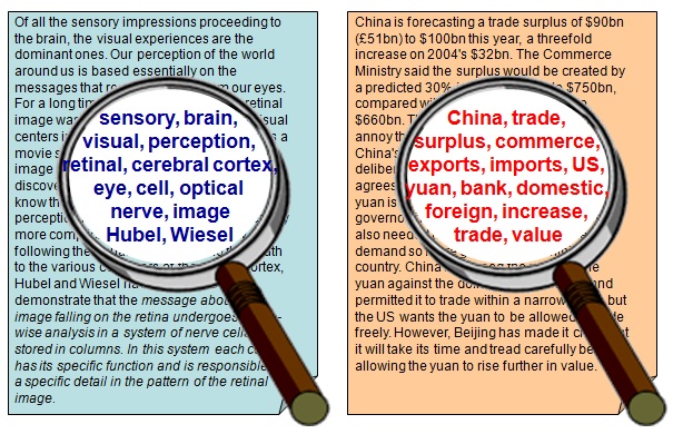
Figure 1: A bag of words model entirely disregards the order of words in a document and simply counts the number of times each word appears. — **Figure 1:** A bag of words model entirely disregards the order of words in a document and simply counts the number of times each word appears.

Treating a document as a “bag of words” allows us to efficiently analyze and compare documents since we do not have to store any information regarding the order and locality of words to each other — we simply count the number of times a word appears in a document, and then use the frequency counts of each word as a method to quantify the document.

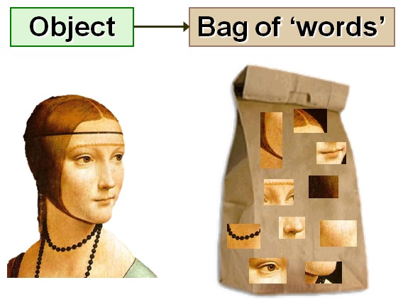
In computer vision, we can apply the same concept — only now instead of working with keywords, our “words” are now image patches and their associated feature vectors:

Figure 2: We take a similar approach in computer vision. Only now instead of actual text words, we count the number of times each image patch occurs. — **Figure 2:** We take a similar approach in computer vision. Only now instead of actual text words, we count the number of times each image patch occurs.

When reading the computer vision literature, it’s common to see the terms bag of words and bag of visual words used interchangeably. Both terms refer to the same concept — representing an image as a collection of unordered image patches; however, I prefer to use the term bag of visual words to alleviate any chance of ambiguity. Using the term bag of words can become especially confusing if you are building a system that fuses both text and image data — imagine the struggle and confusion that can result in trying to explain which “bag” model you are referring to! Because of this, I will use the term bag of visual words, sometimes abbreviated as BOVW throughout the rest of this course.

In Information Retrieval and text analysis, recording the number of times a given word appears in a document is trivially easy — you simply count them and construction a histogram of word occurrences:

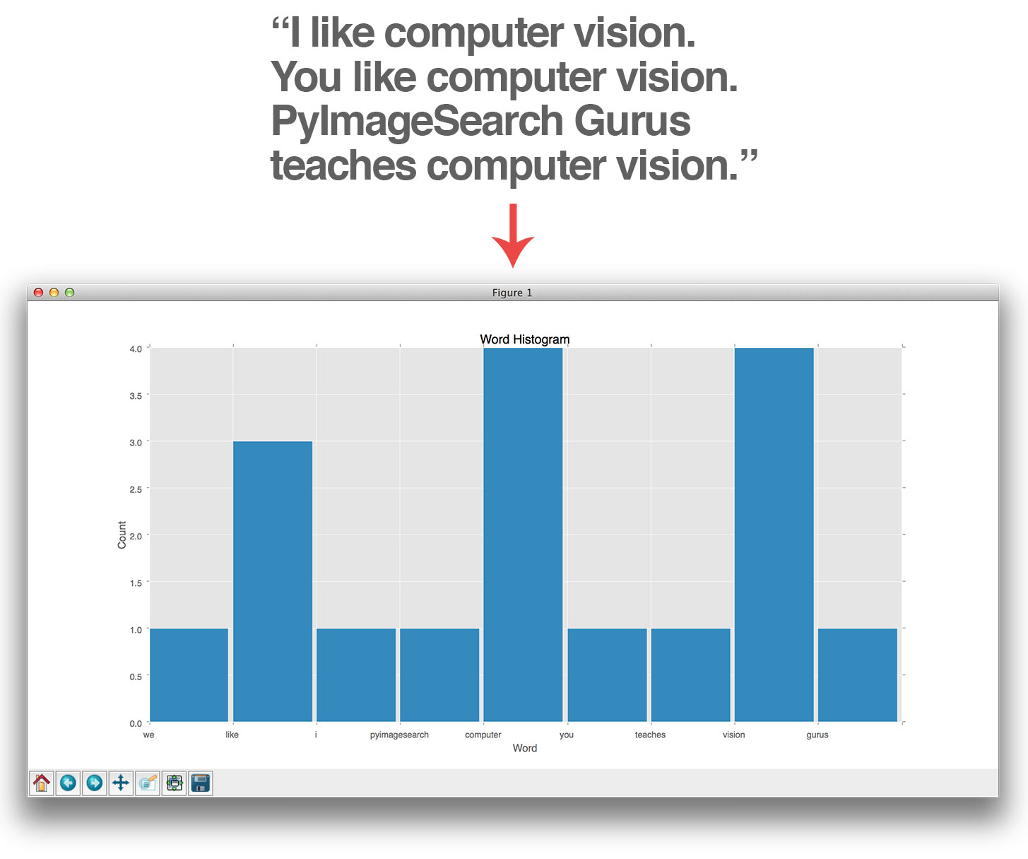
Figure 3: An example of taking a blob of text and converting it into a word histogram. — **Figure 3:** An example of taking a blob of text and converting it into a word histogram.

Here, we can see the word “like” is used twice. The word “teaches” is used only once. And both the words “computer” and “vision” are used four times each. If we were to completely ignore the raw text and simply examine the word occurrence histogram, we could easily determine that this blob of text discusses the topic of “computer vision.”

However, applying the bag of words concept in computer vision is not as simple.

How exactly do you count the number of times an “image patch” appears in an image? And how do you ensure the same “vocabulary” of visual words is used for each image in your dataset?

We’ll discuss the vocabulary problem in more detail later in this lesson, but for the time being let’s assume that through some black-box algorithm that we can construct a large vocabulary (also referred to as a dictionary or codebook; I’ll be using all three terms interchangeably) of possible visual words in our dataset.

Given our dictionary of possible visual words, we can then quantify and represent an image as a histogram which simply counts the number of times each visual word appears. This histogram is our actual bag of visual words:

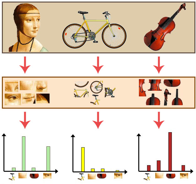
Figure 4: Taking three input images (top), extracting image patches from each of them (middle), and then counting the number of times each visual word appears in the respective images. — **Figure 4:** Taking three input images *(top)*, extracting image patches from each of them *(middle)*, and then counting the number of times each visual word appears in the respective images *(bottom)*.

At the top of this figure, we have three input images of a face, bicycle, and violin. We then extract image patches from each of these objects (middle). Then, on the bottom we take the image patches and use them to construct a histogram that “counts” the number of times each of these image patches appears. These histograms are our actual bag of visual words representation. We call this representation a “bag” because we completely throw out any ordering and locality of image patches and simply tabulate the number of times each type of patch appears.

Notice how the face image has substantially more face patch counts than the other two images. Similarly, the bicycle histogram has many more bicycle patches. And finally, the violin image reports many more violin-like image patches in its histogram.

Building a bag of visual words

Building a bag of visual words can be broken down into a three-step process:

Step #1: Feature extraction
Step #2: Codebook construction
Step #3: Vector quantization.

We will cover each of these steps in detail over the next few lessons, but for the time being, let’s perform a high-level overview of each step.

Step #1: Feature extraction

The first step in building a bag of visual words is to perform feature extraction by extracting descriptors from each image in our dataset.

Feature extraction can be accomplished in a variety of ways including: detecting keypoints and extracting SIFT features from salient regions of our images; applying a grid at regularly spaced intervals (i.e., the Dense keypoint detector) and extracting another form of local invariant descriptor; or we could even extract mean RGB values from random locations in the images.

The point here is that for each image inputted, we receive multiple feature vectors out:

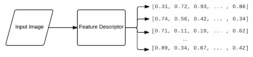
Figure 5: When constructing a bag of visual words, our first step is to apply feature extraction where we extract multiple feature vectors per image. — **Figure 5:** When constructing a bag of visual words, our first step is to apply feature extraction, where we extract multiple feature vectors per image.

Step #2: Dictionary/Vocabulary construction

Now that we have extracted feature vectors from each image in our dataset, we need to construct our vocabulary of possible visual words.

Vocabulary construction is normally accomplished via the k-means clustering algorithm where we cluster the feature vectors obtained from Step #1.

The resulting cluster centers (i.e., centroids) are treated as our dictionary of visual words.

Step #3: Vector quantization

Given an arbitrary image (whether from our original dataset or not), we can quantify and abstractly represent the image using our bag of visual words model by applying the following process:

Extract feature vectors from the image in the same manner as Step #1 above.
For each extracted feature vector, compute its nearest neighbor in the dictionary created in Step #2 — this is normally accomplished using the Euclidean Distance.
Take the set of nearest neighbor labels and build a histogram of length k (the number of clusters generated from k-means), where the i‘th value in the histogram is the frequency of the i‘th visual word. This process in modeling an object by its distribution of prototype vectors is commonly called vector quantization.

An example of constructing a bag of visual words from an image can be seen below:

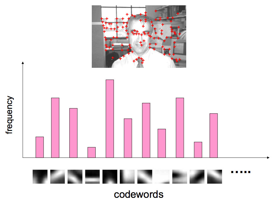
Figure 6: An example of taking an image, detecting keypoints, extracting the features surrounding each keypoint, and then quantizing them according to the closest cluster center. — **Figure 6:** An example of taking an image, detecting keypoints, extracting the features surrounding each keypoint, and then quantizing them according to the closest cluster center.

Finally, given the bag of visual words representation for all images in our dataset, we can apply common machine learning or CBIR algorithms to classify and retrieve images based on their visual contents.

Simply put, the bag of visual words model allows us to take highly discriminate descriptors (such as SIFT), which result in multiple feature vectors per image, and quantize them into a single histogram based on our dictionary. Our image is now represented by a single histogram of discriminative features which can be fed into other machine learning, computer vision, and CBIR algorithms.

Summary

We started this lesson by discussing the bag of words model in text analysis and Information Retrieval. The bag of words models a document by simply counting the number of times a given keyword occurs, irrespective of the ordering of the keywords in the document. The word “bag” is used to describe this method since we ignore the ordering of the keywords.

The same type of concept can be applied in computer vision by counting the number of pre-set image patches occurring in an image — this model is called a bag of visual words.

From there, we discussed the three steps required to construct a bag of visual words, namely: (1) feature extraction; (2) codebook construction, normally via k-means; and (3) vector quantization.

The next four lessons in this module are dedicated to exploring and constructing the bag of visual words model in more detail. First up, extracting keypoints and local invariant descriptors.