In this lesson, we will start to build our actual object detection framework. This framework will consist of many steps and components, including:
- Step #1: Experiment preparation
- Step #2: Feature extraction
- Step #3: Detector training
- Step #4: Non-maxima suppression
- Step #5: Hard negative mining
- Step #6: Detection retraining.
We will have a lesson dedicated to each of these steps in the remainder of this module.
However, let’s start with the first (often overlooked) step — actually setting up our experiment and examining our training data.
It’s important to have an intimate understanding of our training data. The knowledge gained from this initial investigation will guide future parameter choices in our framework. Furthermore, the choices in parameters can either make or break an object detector.
Objectives:
In this lesson, we will:
- Understand the concept of an “Object detection framework”.
- Define a .json file to store framework configurations.
- Explore our training data, allowing us to make critical downstream decisions.
- Explore our “negative images dataset”.
Framework goals
The primary goal of this module is to build an object detection framework that can be used to easily and rapidly build custom object detectors. When building each object detector (e.x., chair, car, airplane, etc.), the code should have to change only minimally, and ideally, not at all.
Specifically, the framework we will be building in the remainder of this module will be capable of constructing an object detector for any object class in the CALTECH-101 dataset.
Below follows the complete directory structure of our framework:
|--- pyimagesearch
|    |---- __init__.py
|    |---- descriptors
|    |    |---- __init__.py
|    |    |---- hog.py
|    |---- object_detection
|    |    |---- __init__.py
|    |    |---- helpers.py
|    |    |---- nms.py
|    |    |---- objectdetector.py
|    |---- utils
|    |    |---- __init__.py
|    |    |---- conf.py
|    |    |---- dataset.py
|--- explore_dims.py
|--- extract_features.py
|--- hard_negative_mine.py
|--- test_model.py
|--- train_model.py
If this seems overwhelming, don’t worry — we’ll be reviewing each of these files (and the role it plays in the framework) in detail.
Modifying the code to construct an object detector for an object class not in this dataset will be extremely easy, and I’ll be sure to point out the required modifications along the way.
In order to maintain cohesive examples in the rest of this module, we’ll be using the car_side data from CALTECH-101, a collection of car images taken from a side view:

Once trained, our object detector will be able to detect the presence (or lack thereof) of a car in an image, followed by drawing a bounding box surrounding it:
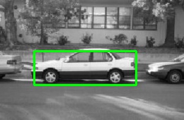
Again, this framework is not specific to side views of cars — it can be used to create any custom object detector of your choice. The car_side choice is simply an example we will use for the next few lessons.
Experiment configurations
Up until now, the vast majority of our code examples have included Python scripts with command line arguments.
The same will be true for our object detection framework, but since (1) we will have a lot of parameters, and (2) many of these parameters will be used over multiple Python scripts, we are going to use a JSON configuration file to store all customizable options of our framework.
There are many benefits to using a JSON configuration file:
- First, we don’t need to explicitly define a never-ending list of command line arguments — all we need to supply is the path to our configuration file.
- A configuration file allows us to consolidate all relevant parameters into a single location.
- This also ensures that we don’t forget which command line options were used for each Python script. All options will be defined within our configuration file.
- Finally, this allows us to have a configuration file for each object detector we want to create. This is a huge advantage and allows us to define object detectors by only modifying a single file.
Below follows the first few lines of our cars.json configuration file:
{
	/****
	* DATASET PATHS
	****/
	"image_dataset": "datasets/caltech101/101_ObjectCategories/car_side",
	"image_annotations": "datasets/caltech101/Annotations/car_side",
	"image_distractions": "datasets/sceneclass13",
...
All we are doing here is defining three sets of data required to train any object detector.
The first, image_dataset , is the path to where our “positive example” images reside on disk. These images should contain examples of the objects we want to learn how to detect — in this case, cars.
The second, image_annotations , is the path to the directory containing the bounding boxes associated with each image in image_dataset .
We need these initial bounding boxes, so we can extract Histogram of Oriented Gradients (HOG) features from their corresponding ROIs and use these features to train our Linear SVM (i.e., the actual “detector”).
Finally, we have our image_distractions , or more simply, the “negative examples” that do not contain any examples of the objects we want to detect. Again, it’s very important that these images do not contain any positive examples — if they do, it can dramatically hurt the performance of our classifier since we are “polluting” our negative training data with examples that should actually be in the positive training set.
A great choice for a distraction dataset is 13 Natural Scene Categories, a collection of natural scenes, including beaches, mountains, forests, etc.
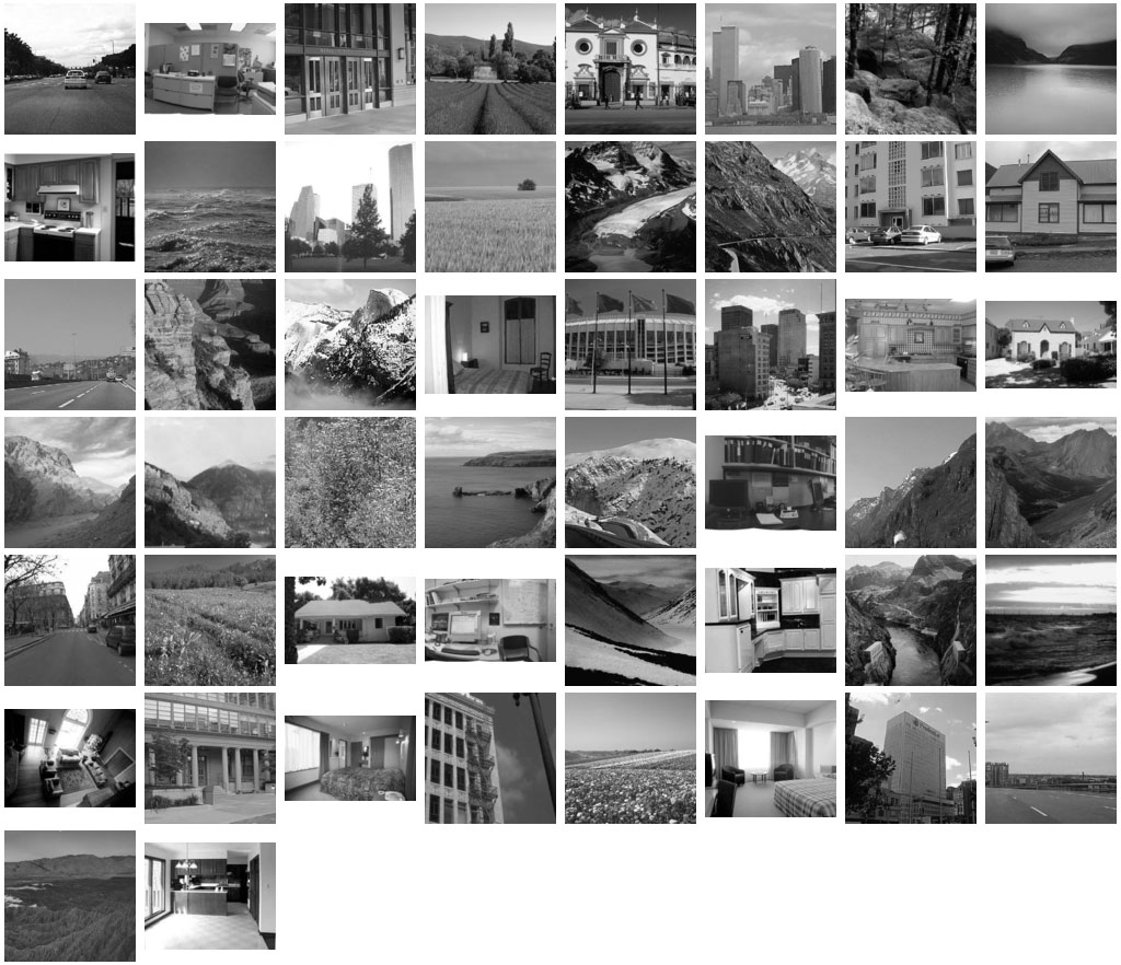
In context of our example, this dataset is sure not to contain any examples of cars.
Exploring our training data
Recall back to our lesson on sliding windows, an object detection tool that is used to “slide” over an image from left-to-right and top-to-bottom. At each window position, HOG features are extracted and then passed on to our classifier to determine if an object of interest resides within that particular window.
However, choosing the appropriate size of our sliding window is a non-trivial problem.
For example, how do we know how wide the window should be? Or how tall? And what is the appropriate aspect ratio (i.e., ratio of width to height) for the objects we want to detect?
The size of our sliding window also has implications on the downstream HOG descriptor.
Again, recall from our lesson on HOG that the descriptor requires (at a bare minimum) two key parameters:
- pixels_per_cell
- cells_per_block
The size of our sliding window can dramatically limit (or dramatically expand) the possible values these parameters can take on.
Since an accurate object detector is highly dependent on our HOG parameter choices, it’s critical that we make a good choice when selecting a sliding window size — a poor choice in sliding window dimensions can almost certainly ensure our object detector will perform poorly.
Given all this pressure on selecting an appropriate sliding window size, it raises the question: “How do we make an informed decision on the dimensions of our sliding window?”
Instead of making a “best guess”, crossing our fingers, and hoping for good results, we can actually examine the dimensions of our object image annotations in order to make a more informed decision.
To accomplish this, let’s define a Python helper script called explore_dims.py :
# import the necessary packages
from __future__ import print_function
from pyimagesearch.utils import Conf
from scipy import io
import numpy as np
import argparse
import glob

# construct the argument parser and parse the command line arguments
ap = argparse.ArgumentParser()
ap.add_argument("-c", "--conf", required=True, help="path to the configuration file")
args = vars(ap.parse_args())
Lines 2-7 handle importing our necessary packages. The Conf class is simply a small helper class that is used to load our .json configuration file from disk.
The contents of conf.py are unexciting and essentially irrelevant to building our custom object detector, but the file is presented below as a matter of completeness:
# import the necessary packages
from json_minify import json_minify
import json

class Conf:
	def __init__(self, confPath):
		# load and store the configuration and update the object's dictionary
		conf = json.loads(json_minify(open(confPath).read()))
		self.__dict__.update(conf)

	def __getitem__(self, k):
		# return the value associated with the supplied key
		return self.__dict__.get(k, None)
(2017-12-9) Update for JSON-minify: This lesson previously made use of the commentjson package which is no-longer supported. The maintainer of commentjson has stopped doing updates and is ignoring pull requests in GitHub. The new, preferred tool is JSON-minify (json_minify ). Take note of the new implementation on Line 8 of conf.py.
If you haven’t already, install JSON-minify:
$ pip install JSON-minify
Lines 10-12 parse our command line arguments. We only need a single switch here, –conf , the path to our JSON configuration file.
Now we are ready to investigate the dimensions of our objects using the supplied annotations in the CALTECH-101 training data:
# load the configuration file and initialize the list of widths and heights
conf = Conf(args["conf"])
widths = []
heights = []

# loop over all annotations paths
for p in glob.glob(conf["image_annotations"] + "/*.mat"):
	# load the bounding box associated with the path and update the width and height
	# lists
	(y, h, x, w) = io.loadmat(p)["box_coord"][0]
	widths.append(w - x)
	heights.append(h - y)

# compute the average of both the width and height lists
(avgWidth, avgHeight) = (np.mean(widths), np.mean(heights))
print("[INFO] avg. width: {:.2f}".format(avgWidth))
print("[INFO] avg. height: {:.2f}".format(avgHeight))
print("[INFO] aspect ratio: {:.2f}".format(avgWidth / avgHeight))
Line 15 loads our configuration, while Lines 16 and 17 initialize the widths and heights of our object bounding boxes.
From there, Line 20 starts looping over the annotation files (which are provided in MATLAB format). Lines 23-25 load the bounding box associated with each annotation file and update the respective width and height lists.
Finally, Lines 28-31 compute the average width and height, along with the aspect ratio of the bounding boxes.
To explore the dimensions of our car side views, just issue the following command:
$ python explore_dims.py --conf conf/cars.json
[INFO] avg. width: 184.46
[INFO] avg. height: 62.01
[INFO] aspect ratio: 2.97
As we can see from the output, the average width of a car is approximately 184px and the average height is 62px, implying that a car is nearly 3x wider than it is tall.
So, now that we know some basic information about our object dimensions, what do we do now?
Is our sliding window size simply 184 x 62?
Not so fast. We need to take into consideration the parameters of our HOG descriptor first — and that’s exactly what our next lesson is going to cover.
Summary
In this lesson, we reviewed the basic structure of our object detection framework. We are going to use JSON configuration files, one config file for each object class we want to detect, that encapsulates all relevant parameters needed to build an object detector.
We also reviewed the entire directory project structure for our object detection framework. This framework can be decomposed into six steps/components. We reviewed the first step in this lesson — preparing your experiment and training data.
In the next lesson, we’ll take the insights gained from the explore_dims.py script and use the average width, average height, and aspect ratio to define the parameters to our HOG descriptor.
Downloads:
Download the CALTECH-101 Dataset