Our last lesson discussed how to use Redis to build an inverted index to facilitate faster (and more scalable) queries to our CBIR system. This lesson will demonstrate how to use our inverted index to perform a search.

By the end of this lesson, you’ll have a fully functioning CBIR system that you can use to scale to very large image datasets. We’ll spend the rest of this module improving our CBIR system.

Objectives:

In this lesson, we will:

Define a Searcher class to pull image IDs out of an inverted index and only explicitly compare (i.e., compute the distance between) images that have a sufficient number of visual words in common.
Apply our Searcher class to perform an actual, optimized search.

Performing a search

Let’s go ahead and take a look at our updated CBIR project directory structure:

|--- pyimagesearch
|    |---- __init__.py
|    |--- db
|    |    |---- __init__.py
|    |    |--- redisqueue.py
|    |--- descriptors
|    |    |---- __init__.py
|    |    |--- detectanddescribe.py
|    |--- indexer
|    |    |---- __init__.py
|    |    |---- baseindexer.py
|    |    |---- bovwindexer.py
|    |    |---- featureindexer.py
|    |--- ir
|    |    |---- __init__.py
|    |    |---- bagofvisualwords.py
|    |    |---- dists.py
|    |    |---- searcher.py
|    |    |---- searchresult.py
|    |    |---- vocabulary.py
|--- build_redis_index.py
|--- cluster_features.py
|--- extract_bvow.py
|--- index_features.py
|--- search.py
|--- visualize_centers.py

We’ve added four new files in this lesson. The first is search.py , the driver Python script used to perform an actual search.

We then have the Searcher class inside the ir sub-module — the Searcher will be used to query the Redis inverted index, pull out candidate images to compare, and then return the final search results.

The searchresults.py and dists.py are simply helper files that we will use along the way. Let’s go ahead and take a look at these helper files.

Helper methods and classes

We’ll start by defining SearchResult , an object used to store:

Our “search results”, or simply, the list of images that are similar to our query image.
Any additional meta-data associated with the search, such as the time it took to perform the search.

Below, we can see the contents of searchresult.py :

# import the necessary packages
from collections import namedtuple

# construct the SearchResult named tuple
SearchResult = namedtuple("SearchResult", ["results", "search_time"])

Now, let’s define the chi2_distance function inside dists.py :

# import the necessary packages
import numpy as np

def chi2_distance(histA, histB, eps=1e-10):
	# compute the chi-squared distance
	d = 0.5 * np.sum(((histA - histB) ** 2) / (histA + histB + eps))

	# return the chi-squared distance
	return d

As the method name suggests, the chi2_distance computes the $\chi^{2}$ between two histograms.

Defining the searcher class

The primary goals of our Searcher class are to:

Use the inverted index to filter images that will have their $\chi^{2}$ distance explicitly computed by only grabbing image indexes that share a significant number of visual words with the query image.
Compare BOVW histograms from the short list of image indexes using the $\chi^{2}$ distance.

That said, let’s see how we are going to accomplish these goals:

# import the necessary packages
from .searchresult import SearchResult
from .dists import chi2_distance
import numpy as np
import datetime
import h5py

class Searcher:
	def __init__(self, redisDB, bovwDBPath, featuresDBPath, idf=None,
		distanceMetric=chi2_distance):
		# store the redis database reference, the idf array, and the distance
		# metric
		self.redisDB = redisDB
		self.idf = idf
		self.distanceMetric = distanceMetric

		# open both the bag-of-visual-words database and the features database
		# for reading
		self.bovwDB = h5py.File(bovwDBPath, mode="r")
		self.featuresDB = h5py.File(featuresDBPath, "r")

On Line 8, we define our Searcher class. The constructor to the Searcher class has three required arguments and two optional ones, each of which we define below:

redisDB : This is our instantiation of the Redis class used to communicate with the Redis data store.
bovwDBPath : The path to our BOVW HDF5 dataset on disk.
featuresDBPath : The path to our raw, extracted keypoints and local invariant descriptors HDF5 dataset.
idf : This optional argument is our inverted document frequency array that counts the number of images a given visual word appears in. We have an entire lesson dedicated to using the inverse document frequency to weight BOVW histograms, so we’ll defer a more thorough explanation of this parameter to a future lesson.
distanceMetric : The distance metric/similarity function used to compare BOVW feature vectors. By default, we’ll use the $\chi^{2}$ distance.

From there, Lines 13-20 store our supplied parameters to the constructor and open the HDF5 datasets.

	def search(self, queryHist, numResults=10, maxCandidates=200):
		# start the timer to track how long the search took
		startTime = datetime.datetime.now()

		# determine the candidates and sort them in ascending order so they can
		# be read from the bag-of-visual-words database
		candidateIdxs = self.buildCandidates(queryHist, maxCandidates)
		candidateIdxs.sort()

		# grab the histograms for the candidates from the bag-of-visual-words
		# database and initialize the results dictionary
		hists = self.bovwDB["bovw"][candidateIdxs]
		queryHist = queryHist.toarray()
		results = {}

		# if the inverse document frequency array has been supplied, multiply the
		# query by it
		if self.idf is not None:
			queryHist *= self.idf

On Line 22, we define our search function, the method that actually kicks off an actual search. This method requires only a single argument, the query BOVW histogram. We can also optionally supply the maximum number of results to return, along with maxCandidates , the maximum number of image indexes to grab from the inverted index that shares a significant number of visual words with the query.

Line 24 starts a timer that we’ll use to keep track of how long a given search takes.

Line 28 makes a call to the buildCandidates method (a function we’ll define shortly), which queries our inverted index and returns a list of candidateIdxs , or more simply, the list of image indexes that shares a significant number of visual words in the query.

Line 29 then takes the candidateIdxs and sorts them in ascending order, allowing us to grab the associated feature vectors from the BOVW HDF5 dataset on Line 33. From there, we convert our sparse queryHist to a dense NumPy array. This conversion of sparse to dense is required to apply our distanceMetric . We’ll also initialize the dictionary of results on Line 35.

Finally, Lines 39 and 40 apply inverse document frequency weighting — a topic that we’ll discuss in a future lesson.

The next step is to compute the distance between the query histogram and the BOVW histograms in the HDF5 dataset:

		# loop over the histograms
		for (candidate, hist) in zip(candidateIdxs, hists):
			# if the inverse document frequency array has been supplied, multiply
			# the histogram by it
			if self.idf is not None:
				hist *= self.idf

			# compute the distance between the histograms and updated the results
			# dictionary
			d = self.distanceMetric(hist, queryHist)
			results[candidate] = d

		# sort the results, this time replacing the image indexes with the image
		# IDs themselves
		results = sorted([(v, self.featuresDB["image_ids"][k], k)
			for (k, v) in results.items()])
		results = results[:numResults]

		# return the search results
		return SearchResult(results, (datetime.datetime.now() - startTime).total_seconds())

On Line 43, we start looping over the histograms in the HDF5 dataset.

Lines 51 and 52 apply the distanceMetric and compute the distance between the query BOVW histogram and the BOVW histogram in our indexed dataset. This distance is then used to update the results dictionary.

Finally, Lines 56 and 57 sort our results , grab the top numResults , and return a SearchResult object to the calling method.

All that’s left for us to do now is define the buildCandidates and finish methods:

	def buildCandidates(self, hist, maxCandidates):
		# initialize the redis pipeline
		p = self.redisDB.pipeline()

		# loop over the columns of the (sparse) matrix and create a query to
		# grab all images with an occurrence of the current visual word
		for i in hist.col:
			p.lrange("vw:{}".format(i), 0, -1)

		# execute the pipeline and initialize the candidates list
		pipelineResults = p.execute()
		candidates = []

		# loop over the pipeline results, extract the image index, and update
		# the candidates list
		for results in pipelineResults:
			results = [int(r) for r in results]
			candidates.extend(results)

		# count the occurrence of each of the canidates and sort in descending
		# order
		(imageIdxs, counts) = np.unique(candidates, return_counts=True)
		imageIdxs = [i for (c, i) in sorted(zip(counts, imageIdxs), reverse=True)]

		# return the image indexes of the candidates
		return imageIdxs[:maxCandidates]

	def finish(self):
		# close the bag-of-visual-words database and the features database
		self.bovwDB.close()
		self.featuresDB.close()

The buildCandidates method requires two arguments: the query histogram, followed by maxCandidates , the maximum number of image indexes to return that shares a significant number of visual words with the query.

Line 65 initializes our Redis pipeline. We then loop over all visual words in the query histogram and construct a Redis operation to grab the image indexes for each of these visual words (Lines 69 and 70).

On Line 73, we execute this pipeline and loop over the results from Redis on Line 78. For each image index returned, we convert the index to an integer and update the candidates list.

Given the candidates list, Lines 84 and 85 count the number of times each image index appears, and sort them (in descending order) according to these counts. Images that share more visual words with the query are placed at the front of the list. And images that share few visual words with the query are placed at the back of the list.

Finally, we return maxCandidates of these image indexes to the calling function.

Putting all the pieces together

The last step in building our image search engine is to define the search.py driver script. This script will be responsible for:

Loading a query image.
Detecting keypoints, extracting local invariant descriptors, and constructing a BOVW histogram.
Querying the Searcher using the BOVW histogram.
Displaying the output results to our screen.

Let’s go ahead and define our search.py file:

# import the necessary packages
from __future__ import print_function
from pyimagesearch.descriptors import DetectAndDescribe
from pyimagesearch.ir import BagOfVisualWords
from pyimagesearch.ir import Searcher
from pyimagesearch.ir import chi2_distance
from pyimagesearch import ResultsMontage
from scipy.spatial import distance
from redis import Redis
from imutils.feature import FeatureDetector_create, DescriptorExtractor_create
import argparse
import pickle
import imutils
import json
import cv2

# construct the argument parser and parse the arguments
ap = argparse.ArgumentParser()
ap.add_argument("-d", "--dataset", required=True, help="Path to the directory of indexed images")
ap.add_argument("-f", "--features-db", required=True, help="Path to the features database")
ap.add_argument("-b", "--bovw-db", required=True, help="Path to the bag-of-visual-words database")
ap.add_argument("-c", "--codebook", required=True, help="Path to the codebook")
ap.add_argument("-i", "--idf", type=str, help="Path to inverted document frequencies array")
ap.add_argument("-r", "--relevant", required=True, help = "Path to relevant dictionary")
ap.add_argument("-q", "--query", required=True, help="Path to the query image")
args = vars(ap.parse_args())

Lines 2-15 import all of our necessary command line arguments — as you can see, there are quite a few classes and methods that are required to perform a search. Lines 18-26 then parse our command line arguments:

–dataset : This is the path to our original UKBench images. We need this path, so we can load results from disk and display them.
–features-db : The path to our raw keypoints and local invariant descriptors HDF5 dataset.
–bovw-db : The path to our BOVW HDF5 dataset.
–codebook : Here, we specify the path to our cPickle ‘d vocabulary of visual words, resulting from the clustering features phase.
–idf : We can optionally specify our inverted index array, but we’ll simply ignore this switch for now.
–relevant : For each image in the UKBench dataset, there are four images considered to be “relevant” to it. The –relevant path contains the path to the .json file that holds these relevant mappings, allowing us to determine the accuracy of our CBIR system.
–query : Finally, we must specify the path to our query image.

Let’s continue to move through the search.py script:

# initialize the keypoint detector, local invariant descriptor, descriptor pipeline,
# distance metric, and inverted document frequency array
detector = FeatureDetector_create("SURF")
descriptor = DescriptorExtractor_create("RootSIFT")
dad = DetectAndDescribe(detector, descriptor)
distanceMetric = chi2_distance
idf = None

# if the path to the inverted document frequency array was supplied, then load the
# idf array and update the distance metric
if args["idf"] is not None:
	idf = pickle.loads(open(args["idf"], "rb").read())
	distanceMetric = distance.cosine

# load the codebook vocabulary and initialize the bag-of-visual-words transformer
vocab = pickle.loads(open(args["codebook"], "rb").read())
bovw = BagOfVisualWords(vocab)

Lines 30-34 initialize our Fast Hessian and RootSIFT descriptor pipeline. We’ll also initialize our distanceMetric to be the $\chi^{2}$ distance.

Provided a path to the inverted document frequency array was provided, we’ll load it from disk on Lines 38-40.

Finally, Lines 43 and 44 load our visual vocab from disk and initialize the BagOfVisualWords quantizer.

We are now ready to load our query image and describe it:

# load the relevant queries dictionary and lookup the relevant results for the
# query image
relevant = json.loads(open(args["relevant"]).read())
queryFilename = args["query"][args["query"].rfind("/") + 1:]
queryRelevant = relevant[queryFilename]

# load the query image and process it
queryImage = cv2.imread(args["query"])
cv2.imshow("Query", imutils.resize(queryImage, width=320))
queryImage = imutils.resize(queryImage, width=320)
queryImage = cv2.cvtColor(queryImage, cv2.COLOR_BGR2GRAY)

# extract features from the query image and construct a bag-of-visual-words from it
(_, descs) = dad.describe(queryImage)
hist = bovw.describe(descs).tocoo()

On Line 53, we load our image from disk. We then resize it to have a maximum width of 320 pixels, and convert it to grayscale (Lines 55 and 56).

Lines 59 and 60 detect keypoints and extract local invariant descriptors from our query, then we use these descriptors to construct a BOVW histogram.

Finally, we are ready to perform a search:

# connect to redis and perform the search
redisDB = Redis(host="localhost", port=6379, db=0)
searcher = Searcher(redisDB, args["bovw_db"], args["features_db"], idf=idf,
	distanceMetric=distanceMetric)
sr = searcher.search(hist, numResults=20)
print("[INFO] search took: {:.2f}s".format(sr.search_time))

# initialize the results montage
montage = ResultsMontage((240, 320), 5, 20)

# loop over the individual results
for (i, (score, resultID, resultIdx)) in enumerate(sr.results):
	# load the result image and display it
	print("[RESULT] {result_num}. {result} - {score:.2f}".format(result_num=i + 1,
		result=resultID, score=score))
	result = cv2.imread("{}/{}".format(args["dataset"], resultID))
	montage.addResult(result, text="#{}".format(i + 1),
		highlight=resultID in queryRelevant)

# show the output image of results
cv2.imshow("Results", imutils.resize(montage.montage, height=700))
cv2.waitKey(0)
searcher.finish()

On Line 63, we connect to Redis so we can access our inverted index. The actual search is then performed on Lines 64-66 using our Searcher class. The remainder of the search.py script loops over the results, adds them to our output image, and displays the final result set to our screen.

Running our CBIR system

Before we can perform a search, we first need to start Redis:

$ ./redis-server

Note: Make sure you have already executed build_redis_index.py before calling search.py . If you do not, you’ll get an error message that may leave you scratching your head.

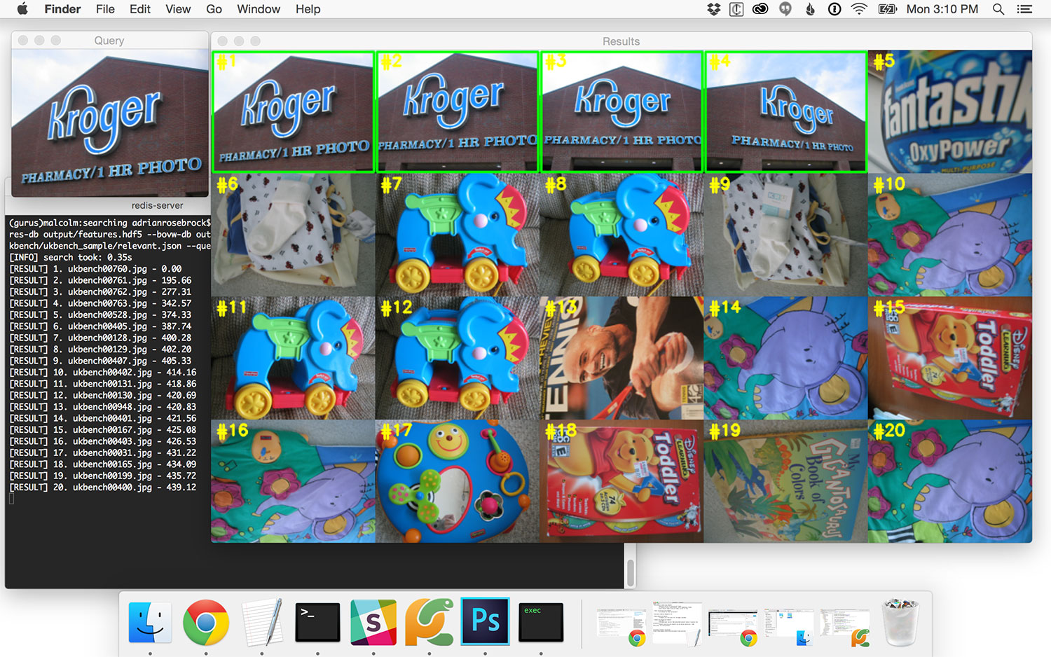
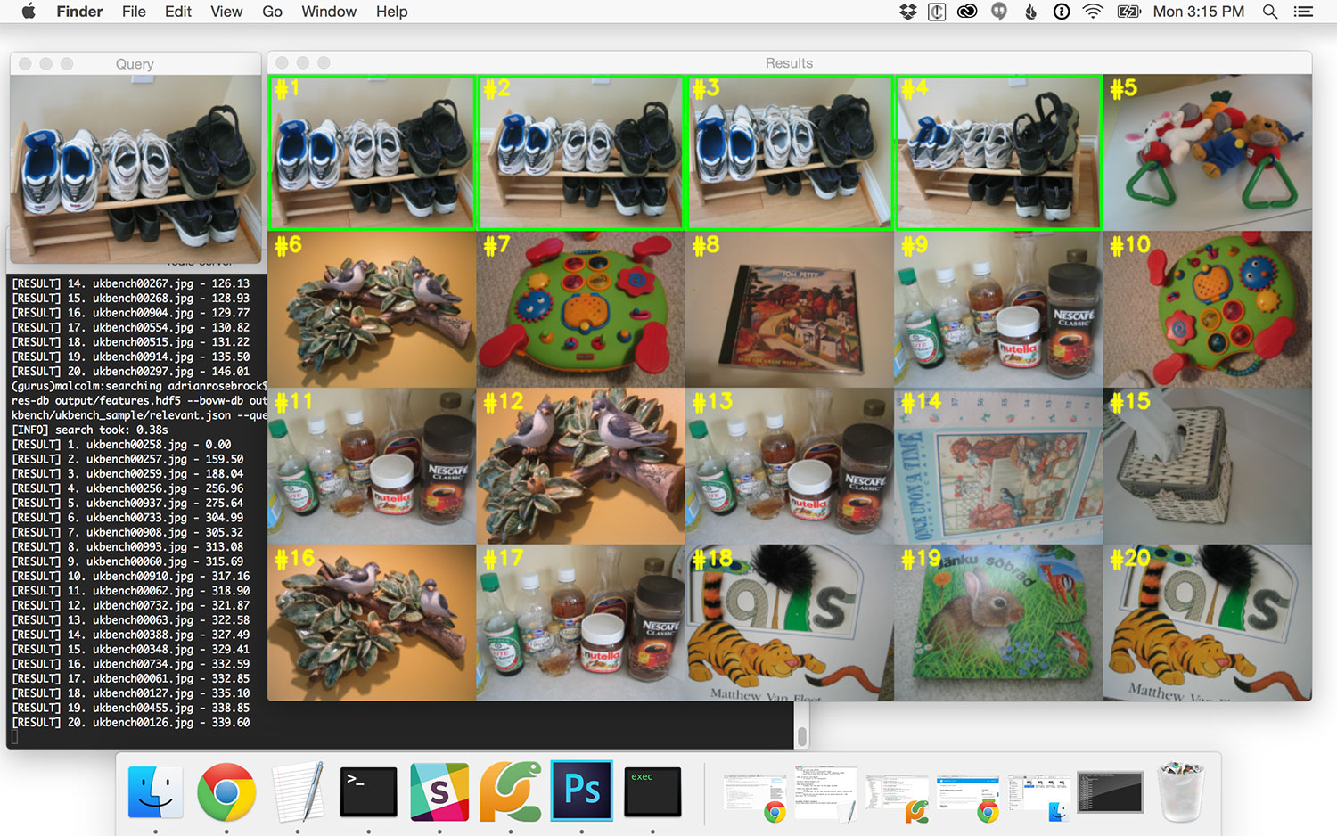
Now that Redis is up and running, just issue the following command to test out our fully functioning CBIR system:

$ python search.py --dataset ../ukbench --features-db output/features.hdf5 --bovw-db output/bovw.hdf5 \
	--codebook output/vocab.cpickle --relevant ../ukbench/relevant.json --query ../ukbench/ukbench00258.jpg

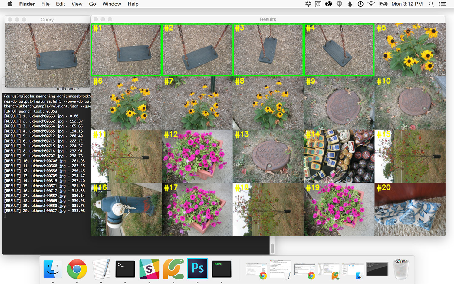
Figure 1: Using our rack of shoes image as our query, we are able to find the four relevant images also containing the rack of shoes in our database. — **Figure 1:** Using our rack of shoes image as our query, we are able to find the four relevant images also containing the rack of shoes in our database.

In this next command, we find the four relevant images containing a seat on a child’s swing set:

$ python search.py --dataset ../ukbench --features-db output/features.hdf5 --bovw-db output/bovw.hdf5 \
	--codebook output/vocab.cpickle --relevant ../ukbench/relevant.json --query ../ukbench/ukbench00653.jpg

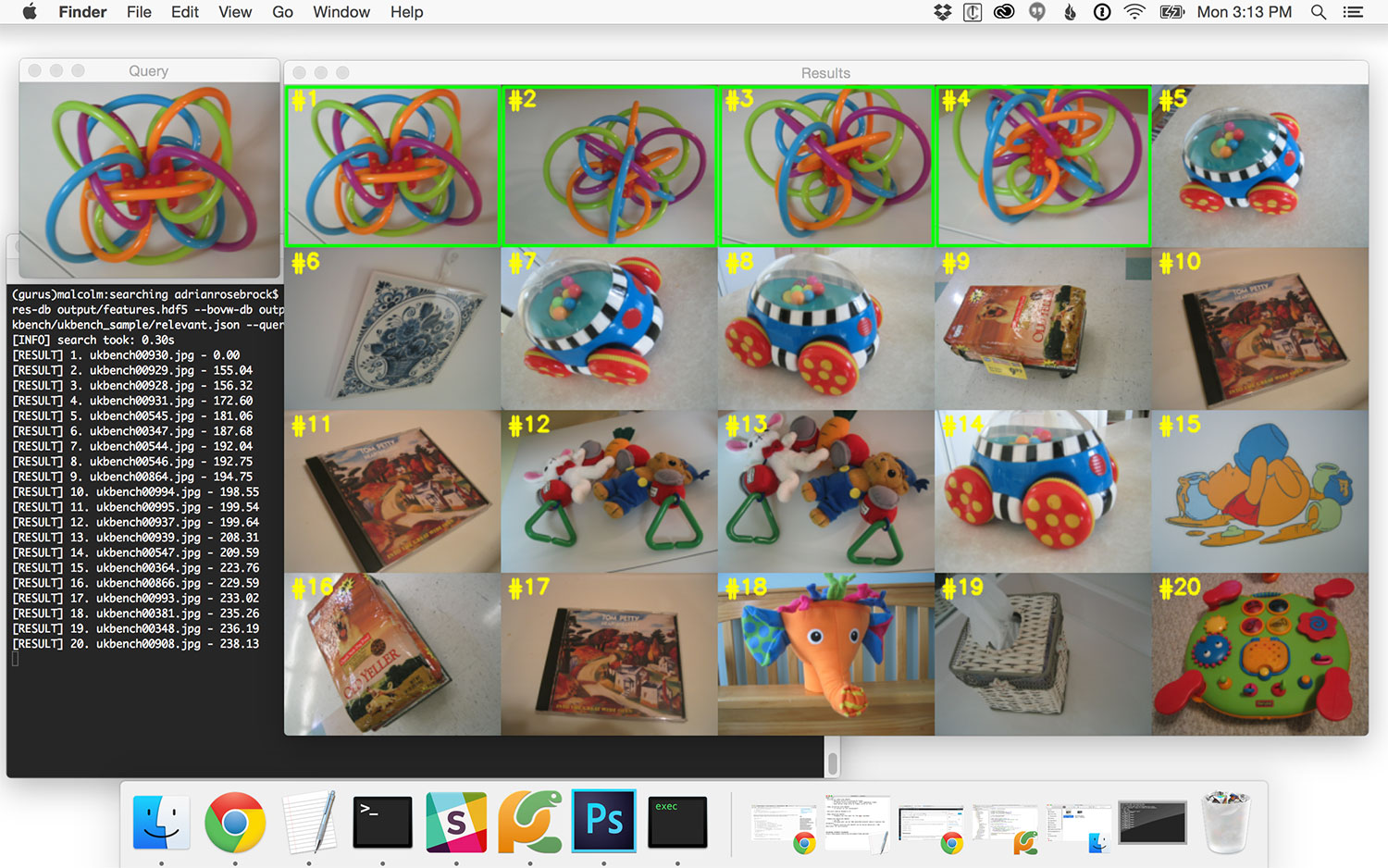
Figure 2: Finding all images in the UKBench dataset containing a child swing set seat. — **Figure 2:** Finding all images in the UKBench dataset containing a child’s swing set seat.

Let’s give one last query image a try:

$ python search.py --dataset ../ukbench --features-db output/features.hdf5 --bovw-db output/bovw.hdf5 \
	--codebook output/vocab.cpickle --relevant ../ukbench/relevant.json --query ../ukbench/ukbench00928.jpg

Figure 3: Here we present our CBIR system with a multi-colored child's toy -- our image search engine is able to find all four relevant images in response to our query image. — **Figure 3:** Here, we present our CBIR system with a multi-colored child’s toy — our image search engine is able to find all four relevant images in response to our query image.

Summary

In this lesson, we put together all the pieces from previous lessons and built a fully functioning CBIR system. Not only is this CBIR system accurate, but it’s also scalable, since it leverages an inverted index.

Unlike previous image search engines we have built, which relied on performing a linear search (i.e., looping over every feature vector in our dataset and explicitly computing the distance between it and the query histogram), we can now use the inverted index to grab a subset of relevant images and perform a ranking of these images using our distance metric.

While we visually demonstrated that our CBIR system is capable of returning relevant results, the question still remains: “How do we obtain a single number that represents the ‘accuracy’ of our CBIR system?”

The answer to this question varies from dataset to dataset, but in our next lesson, I’ll demonstrate how to evaluate our CBIR system on the UKBench dataset, leaving us with a single number to quantify the “accuracy” of our image search engine.

Downloads:

Download the Code