Figure 6: Our k-NN classifier is able to correctly recognize the digit "6". — **Figure 6:** Our k-NN classifier is able to correctly recognize the digit “6”.

We’ve spent a decent amount of time discussing the image classification in this module. We’ve learned about the challenges. The types of learning algorithms we can use. And even the general pipeline that is used to build any image classifier.

But we have yet to really build an image classifier of our own.

Today, that is all going to change.

We’re going to start this lesson by reviewing the simplest image classification algorithm: k-Nearest Neighbor (k-NN). This algorithm is so simple that it doesn’t do any actual “learning” — yet it is still heavily used in many computer vision algorithms. And as you’ll see, we’ll be able to utilize this algorithm to recognize handwritten digits from the popular MNIST dataset.

Objectives:

By the end of this lesson, you will:

Have an understanding of the k-Nearest Neighbor classifier.
Know how to apply the k-Nearest Neighbor classifier to image datasets.
Understand how the value of k impacts classifier performance.
Be able to recognize handwritten digits from (a sample of) the MNIST dataset.

The k-Nearest Neighbor Classifier

The k-Nearest Neighbor classifier is by far the most simple image classification algorithm. In fact, it’s so simple that it doesn’t actually “learn” anything! Instead, this algorithm simply relies on the distance between feature vectors, much like in building an image search engine — only this time, we have the labels associated with each image, so we can predict and return an actual category for the image.

Simply put, the k-NN algorithm classifies unknown data points by finding the most common class among the k closest examples. Each data point in the k closest data points casts a vote, and the category with the highest number of votes wins! Or in plain english: “Tell me who your neighbors are, and I’ll tell you who you are”.

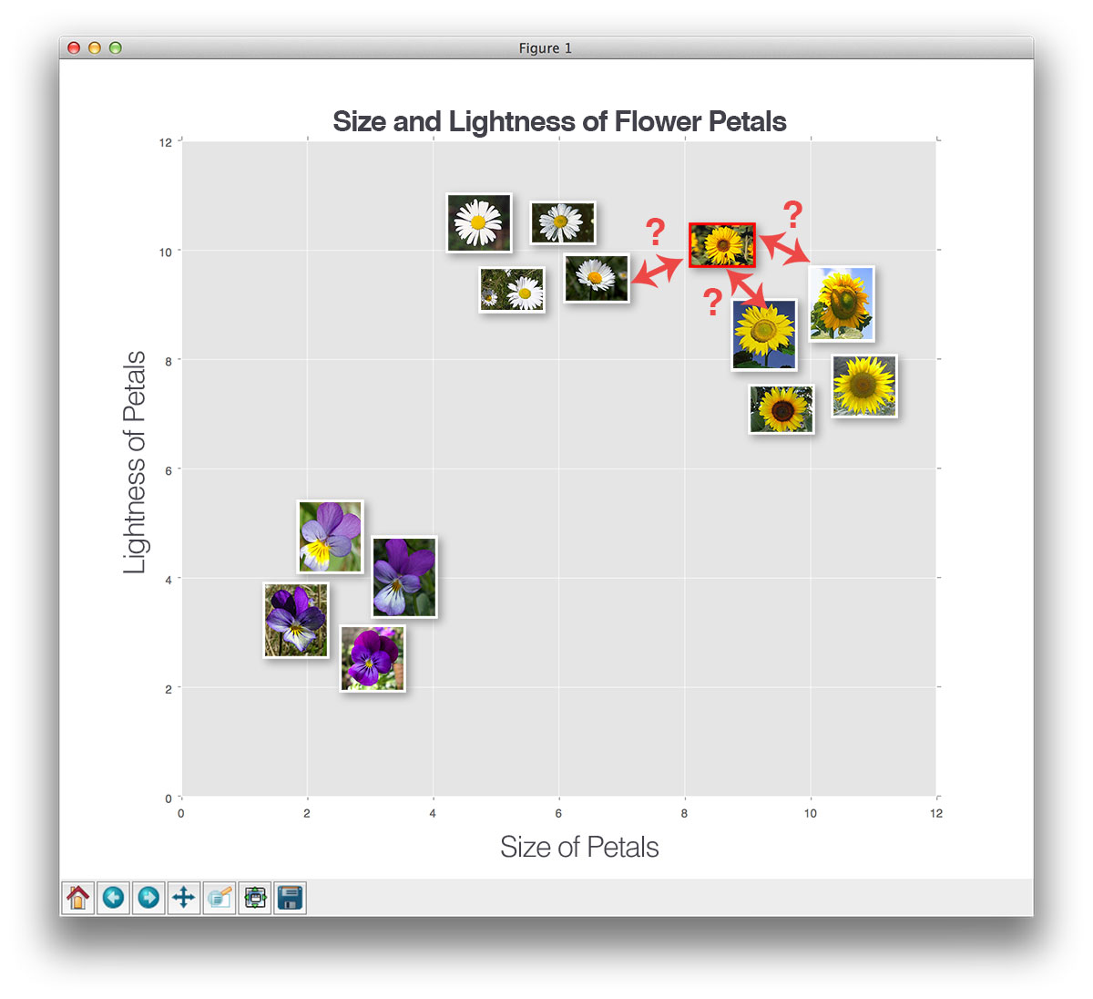
Figure 1: Given a dataset of flowers, how might we classify the the outlined in red? — **Figure 1:** Given a dataset of flowers, how might we classify the image outlined in red?

In order for the k-NN algorithm to work, it makes the primary assumption that feature vectors that lie close together in an n-dimensional space have similar visual contents:

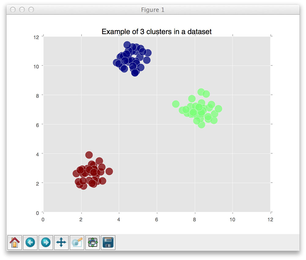
Figure X: — **Figure 2:** A visual example of three distinct “clusters” of data.

Here, we can see three categories of images, denoted as red, blue, and green dots, respectively. We can see that each of these sets of data points are grouped relatively close together in our n-dimensional space. This implies that the distance between two red dots is much smaller than the distance between a red dot and a blue dot.

However, in order to apply the k-Nearest Neighbor classifier, we first need to select a distance metric or a similarity function. We briefly discussed the Euclidean distance (often called the L2-distance) in our lesson on color channel statistics:

$d(\boldsymbol{p},\boldsymbol{q}) = \sqrt{\sum_{i-1}^{N}(q_{i} - p_{i})^{2}}$

But many other distance metrics exist including the Manhattan/city block distance (often called the L1-distance):

$d(\boldsymbol{p},\boldsymbol{q}) = \sum_{i-1}^{N}|q_{i} - p_{i}|$

Note: For more information on $L^{P}$ spaces, give this page a read.

In reality, you can use whichever distance metric/similarity function most suits your data (and gives you the best classification results). However, for the remainder of this lesson, we’ll be using the most popular distance metric: the Euclidean distance.

k-NN in action

At this point, we understand the principles of the k-NN algorithm. We know that it relies on the distance between feature vectors to make a classification. And we know that it requires a distance metric/similarity function to compute these distances.

But how do we actually make the classification?

To answer this question, let’s look at the following figure:

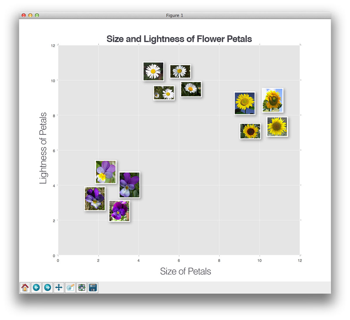
Figure 2: An example of plotting three species of flowers according to the size and lightness of their petals. — **Figure 3:** An example of plotting three species of flowers according to the size and lightness of their petals.

Here, we have a dataset of three types of flowers — sunflowers, daises, and pansies — and we have plotted them according to the size and lightness of their petals.

Now, let’s insert a new, unknown flower and try to classify it using only a single neighbor (i.e. k=1):

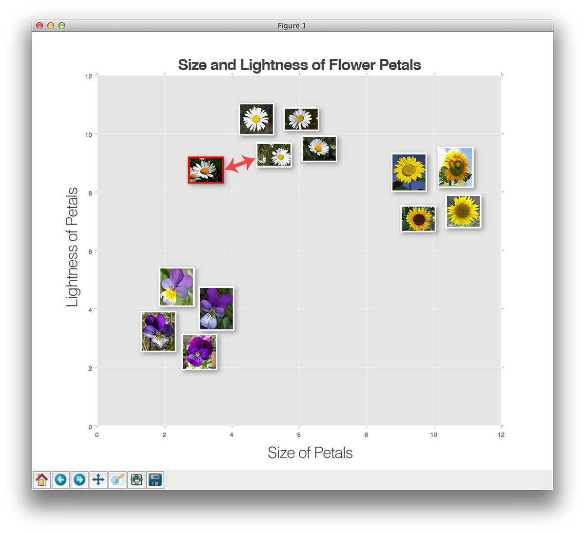
Figure 3: In this example we insert an unknown image (highlighted as red) into the dataset and then use the distance between the unknown flower and dataset of flowers to make the classification. — **Figure 4:** In this example, we insert an unknown image (highlighted as red) into the dataset and then use the distance between the unknown flower and dataset of flowers to make the classification.

Here, we have found the “nearest neighbor” to our test flower, indicated by k=1. And according to the label of the nearest flower, it’s a daisy.

Let’s try another “unknown flower”, this time using k=3:

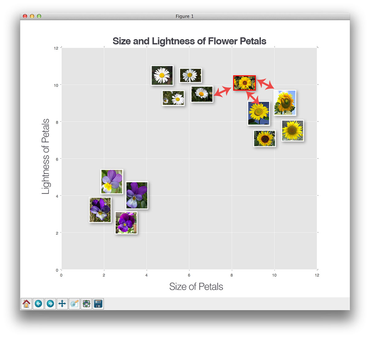
Figure 4: Let's classify another flower -- only this time let's use k=3 neighbors rather than just k=1. — **Figure 5:** Let’s classify another flower — only this time let’s use *k=3* neighbors rather than just *k=1*.

This time, we have found two sunflowers and one daisy in the top three results. Since the sunflower category has the largest number of votes, we’ll classify this unknown flower as a sunflower.

We can keep performing this process for varying values of k, but no matter how large or small k becomes, the principle remains the same — the category with the largest number of votes in the k closest training points wins and is used as the label for the testing point.

Hyperparameter tuning

There are two clear parameters that we are concerned with when running the k-NN algorithm. The first is obvious: the value of k. What is the optimal value of k? If it’s too small (such as when k=1), then we gain efficiency, but become susceptible to noise and outlier data points. However, if k is too large, then we are at risk for over-smoothing our classification results and increasing bias.

The second parameter we should consider tuning is the actual distance metric. Is the Euclidean distance the best choice? What about the Manhattan distance? Or $\chi^2$ ?

To handle this problem, we need to follow Step 2 of our image classification pipeline and split our data into three sets: a training set, a validation set, and a testing set.

Using this three-split scheme we can:

Train our classifier on the training data using various values of k (and various distance functions, if we wish).
Evaluate the performance on the classifier on the validation set, keeping track of which parameters obtained the highest accuracy.
Take the parameters that obtained the highest accuracy and train our k-NN classifier using those parameters.
Evaluate our “best” classifier on the test set and obtain our final results.

Again, by using this scheme, we are able to try various parameter values, find the set of parameters that gives the best performance, and then finally evaluate our classifier in an un-biased (and fair) manner.

Now that we understand the basics of the k-NN algorithm, let’s apply it to recognize handwritten digits from the MNIST dataset.

Recognizing handwritten digits using MNIST

Figure 5: A sample of the MNIST data for handwritten digit recognition. — **Figure 6:** A sample of the MNIST data for handwritten digit recognition.

In the remainder of this lesson, we’ll be using the k-Nearest Neighbor classifier to classify images from the MNIST dataset, which consists of handwritten digits. The MNIST dataset is one of the most well studied datasets in the computer vision and machine learning literature. In many cases, it’s a benchmark and a standard to which machine learning algorithms are ranked.

The goal of this dataset is to correctly classify the handwritten digits 0-9. Instead of utilizing the entire dataset (which consists of 60,000 training images and 10,000 testing images,) we’ll be using a small subset of the data provided by the scikit-learn library — this subset includes 1,797 digits, which we’ll split into training, validation, and testing sets, respectively.

Each image in the 1,797-digit dataset from scikit-learn is represented as a 64-dim raw pixel intensity feature vector. This means that each image is actually an 8 x 8 grayscale image, but scikit-learn “flattens” the image into a list.

All digits are placed on a black background with the foreground being shades of white and gray.

Our goal here is to train a k-NN classifier on the raw pixel intensities and then classify unknown digits.

To accomplish this goal, we’ll be using our five-step pipeline to train image classifiers:

Step 1 – Structuring our initial dataset: Our initial dataset consists of 1,797 digits representing the numbers 0-9. These images are grayscale, 8 x 8 images with digits appearing as white on a black background. These digits have also been heavily pre-processed, aligned, and centered, making our classification job slightly easier.
Step 2 – Splitting the dataset: We’ll be using three splits for our experiment. The first set is our training set, used to train our k-NN classifier. We’ll also use a validation set to find the best value for k. And we’ll finally evaluate our classifier using the testing set.
Step 3 – Extracting features: Instead of extracting features to represent and characterize each digit (such as HOG, Zernike Moments, etc), we’ll instead use just the raw, grayscale pixel intensities of the image.
Step 4 – Training our classification model: Our k-NN classifier will be trained on the raw pixel intensities of the images in the training set. We’ll then determine the best value of k using the validation set.
Step 5 – Evaluating our classifier: Once we have found the best value of k, we can then evaluate our k-NN classifier on our testing set.

Let’s go ahead and get this example started. Open up a new file, name it mnist_demo.py , and let’s get coding:

# import the necessary packages
from __future__ import print_function
from sklearn.neighbors import KNeighborsClassifier
from sklearn.metrics import classification_report
from sklearn import datasets
from skimage import exposure
import numpy as np
import imutils
import cv2
import sklearn

# handle older versions of sklearn
if int((sklearn.__version__).split(".")[1]) < 18:
	from sklearn.cross_validation import train_test_split

# otherwise we're using at lease version 0.18
else:
	from sklearn.model_selection import train_test_split

# load the MNIST digits dataset
mnist = datasets.load_digits()

# take the MNIST data and construct the training and testing split, using 75% of the
# data for training and 25% for testing
(trainData, testData, trainLabels, testLabels) = train_test_split(np.array(mnist.data),
	mnist.target, test_size=0.25, random_state=42)

# now, let's take 10% of the training data and use that for validation
(trainData, valData, trainLabels, valLabels) = train_test_split(trainData, trainLabels,
	test_size=0.1, random_state=84)

# show the sizes of each data split
print("training data points: {}".format(len(trainLabels)))
print("validation data points: {}".format(len(valLabels)))
print("testing data points: {}".format(len(testLabels)))

The first thing we’ll do is import our necessary packages on Lines 2-18. The most important imports to take note of are:

Line 3: The KNeighborsClassifier is our implementation of the k-NN algorithm, again provided by scikit-learn.
Line 4: The classification_report function is a handy little tool that will help us evaluate the performance of our classifier.
Line 5: The datasets sub-module of scikit-learn will allow us to load our MNIST dataset.
Lines 13-18: We’ll import the train_test_split function, which is a convenience function provided by scikit-learn to help us create training and testing splits of our data.

(2018-01-12) Update for sklearn: The sklearn.cross_validation module is deprecated in version sklearn==0.18 and replaced with sklearn.model_selection . The sklearn.cross_validation module will no-longer be available in sklearn==0.20 .

From there, we go ahead and load the MNIST dataset sample on Line 21. We’ll also create our training testing split on Lines 25 and 26, using 75% of the data for training and the remaining 25% for testing.

However, we also need a validation set so we can tune the value of k. We create our validation set on Lines 29 and 30 by partitioning our training data — 10% of the training data will be allocated to validation, while the remaining 90% will remain as training data.

Finally, Lines 33-35 show the size of each of our data splits:

training data points: 1212
validation data points: 135
testing data points: 450

Here, we can see we are using X images for training, Y values for validation, and Z values for testing.

Now that we have our data splits taken care of, let’s train our classifier and find the optimal value of k:

# initialize the values of k for our k-Nearest Neighbor classifier along with the
# list of accuracies for each value of k
kVals = range(1, 30, 2)
accuracies = []

# loop over various values of `k` for the k-Nearest Neighbor classifier
for k in range(1, 30, 2):
	# train the k-Nearest Neighbor classifier with the current value of `k`
	model = KNeighborsClassifier(n_neighbors=k)
	model.fit(trainData, trainLabels)

	# evaluate the model and update the accuracies list
	score = model.score(valData, valLabels)
	print("k=%d, accuracy=%.2f%%" % (k, score * 100))
	accuracies.append(score)

# find the value of k that has the largest accuracy
i = int(np.argmax(accuracies))
print("k=%d achieved highest accuracy of %.2f%% on validation data" % (kVals[i],
	accuracies[i] * 100))

On Line 39, we define the list of k values that we want to try, which consist of the odd numbers between the range [1, 30] (any guesses as to why we use odd numbers?).

We then loop over each of these values of k and train a KNeighborsClassifier on Lines 45 and 46, supplying your training data and training labels to the fit method of the model .

After our model is trained, we need to evaluate it using our validation data (Line 49). The score method of our model checks to see how many predictions our k-NN classifier got right (the higher the score, the better, indicating that the classifier correctly labeled the digit a higher percentage of the time). Next we take this score and update our list of accuracies so we can determine the value of k that achieved the highest accuracy on the validation set (Lines 54-56).

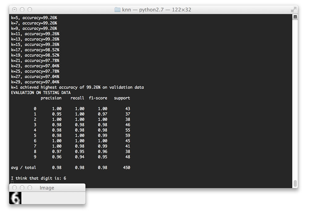
Running our Python script, you’ll see the following output from parameter tuning phase:

k=1, accuracy=99.26%
k=3, accuracy=99.26%
k=5, accuracy=99.26%
k=7, accuracy=99.26%
k=9, accuracy=99.26%
k=11, accuracy=99.26%
k=13, accuracy=99.26%
k=15, accuracy=99.26%
k=17, accuracy=98.52%
k=19, accuracy=98.52%
k=21, accuracy=97.78%
k=23, accuracy=97.04%
k=25, accuracy=97.78%
k=27, accuracy=97.04%
k=29, accuracy=97.04%
k=1 achieved highest accuracy of 99.26% on validation data

Notice how the values of k=1 to k=15 all obtained the same accuracy. However, computing the distance to only a single neighbor is substantially more efficient, thus we will use k=1 to train and evaluate our classifier on the final testing data:

# re-train our classifier using the best k value and predict the labels of the
# test data
model = KNeighborsClassifier(n_neighbors=kVals[i])
model.fit(trainData, trainLabels)
predictions = model.predict(testData)

# show a final classification report demonstrating the accuracy of the classifier
# for each of the digits
print("EVALUATION ON TESTING DATA")
print(classification_report(testLabels, predictions))

The code here is fairly straightforward: we are simply taking the value of k that achieved the highest accuracy, re-training our KNeighborsClassifier using this value of k, and then evaluating the performance using the classification_report function, the output of which you can see below:

EVALUATION ON TESTING DATA
             precision    recall  f1-score   support

          0       1.00      1.00      1.00        43
          1       0.95      1.00      0.97        37
          2       1.00      1.00      1.00        38
          3       0.98      0.98      0.98        46
          4       0.98      0.98      0.98        55
          5       0.98      1.00      0.99        59
          6       1.00      1.00      1.00        45
          7       1.00      0.98      0.99        41
          8       0.97      0.95      0.96        38
          9       0.96      0.94      0.95        48

avg / total       0.98      0.98      0.98       450

Wow, 98% accuracy! That’s quite high! Furthermore, we can see the digits 0, 2, 6, and 7 are classified correctly 100% of the time. The digit 1 obtains the lowest classification accuracy of 95%.

So given this high classification accuracy, does this mean that we have “solved” handwritten digit recognition? Unfortunately, no — it does not. While the MNIST dataset is well known and heavily used as a benchmark, it doesn’t necessarily translate into real-world viability. This is mainly due to the dataset itself, where each and every image has been heavily pre-processed — including cropping, perfect thresholding, and centered.

In the real world, your dataset will never be as “nice” and cleanly pre-processed as the MNIST dataset. And as we’ll find out in our case study on real-world handwriting recognition, we’ll need to extract feature vectors from each digit rather than relying on the raw pixel intensities of the image. With that said, it’s still useful to see how computing the Euclidean distance between raw pixel intensities can lead to high accuracy classifiers provided that the dataset has been appropriately pre-processed.

Finally, let’s end this code example by examining some of the individual predictions from our k-NN classifier:

# loop over a few random digits
for i in list(map(int, np.random.randint(0, high=len(testLabels), size=(5,)))):
	# grab the image and classify it
	image = testData[i]
	prediction = model.predict(image.reshape(1, -1))[0]

	# convert the image for a 64-dim array to an 8 x 8 image compatible with OpenCV,
	# then resize it to 32 x 32 pixels so we can see it better
	image = image.reshape((8, 8)).astype("uint8")
	image = exposure.rescale_intensity(image, out_range=(0, 255))
	image = imutils.resize(image, width=32, inter=cv2.INTER_CUBIC)

	# show the prediction
	print("I think that digit is: {}".format(prediction))
	cv2.imshow("Image", image)
	cv2.waitKey(0)

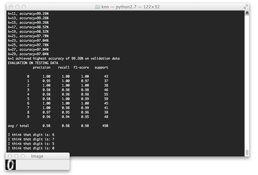
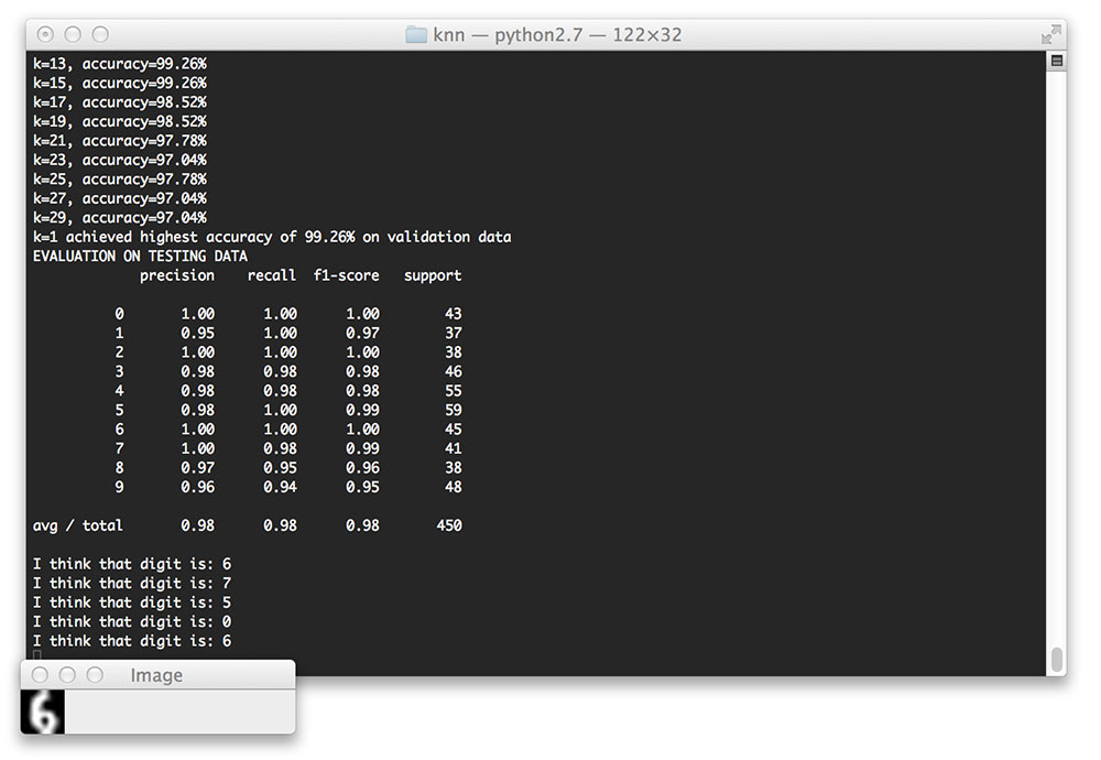
On Line 70, we loop over five random images from our testing set. Line 73 takes the random image and predict what digit the image contains. Finally, Lines 77-79 reshape the 64-dim raw pixel intensity feature vector to an 8 x 8 image, which we blow up to 32 x 32 pixels, so we can better visualize it.

Here are a few examples of individual classifications from our mnist_demo.py script:

Let’s give another one a try:

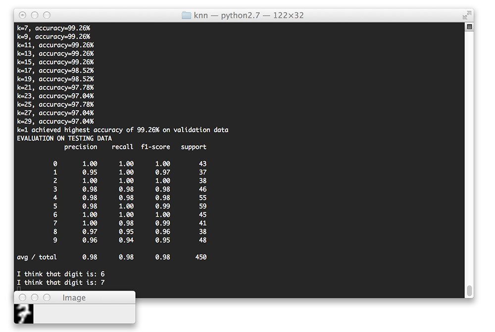
Figure 7: Simply computing the Euclidean distance between raw pixel intensities of the images allows us to correctly classify the handwritten digit "7". — **Figure 8:** Simply computing the Euclidean distance between raw pixel intensities of the images allows us to correctly classify the handwritten digit “7”.

Here’s another sample, this one being more skewed and distorted than the others:

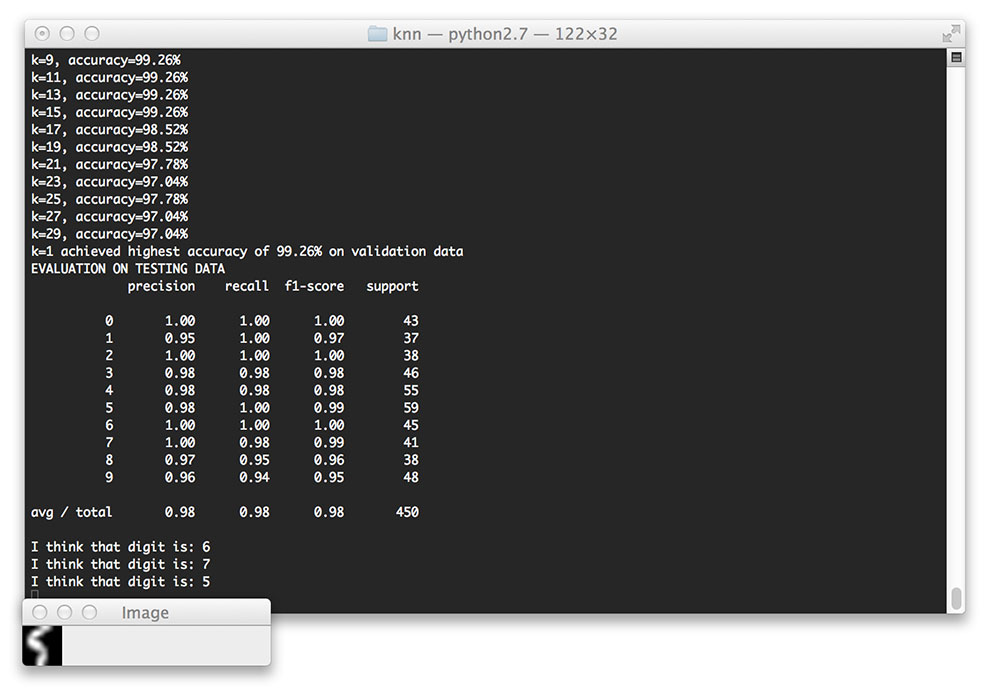
Figure 8: Even though the "5" is skewed and distorted, we can still recognize it. — **Figure 9:** Even though the “5” is skewed and distorted, we can still recognize it.

The digit “0” is also not a problem for our classifier:

Figure 9: Another example of our k-NN classifier in action. — **Figure 10:** Another example of our k-NN classifier in action.

One last example:

Figure 10: The digit "6" is also trivially easy for our k-NN classifier. — **Figure 11:** The digit “6” is also easy for our k-NN classifier.

Pros and Cons of k-NN

Before we wrap up this lesson, we should first discuss some of the advantages and disadvantages of the k-NN classifier.

One main advantage of the k-NN algorithm is that it’s extremely simple to implement and understand. Furthermore, the classifier takes absolutely no time to train, since all we need to do is store our data points for the purpose of later computing distances to them and obtaining our final classification.

However, we pay for this simplicity at classification time. Classifying a new testing data point requires a comparison to every single data point in our training data, which scales $O(N)$ , making working with large datasets computationally prohibitive. We can combat this problem by using Approximate Nearest Neighbor (ANN) algorithms (such as kd-trees, FLANN, and random projections, etc.); however, this requires that we trade space/time complexity for the the “correctness” of our nearest neighbor algorithm, since we are performing an approximation. That said, in many cases it is well worth the effort and small loss in accuracy to use the k-NN algorithm. This is in contrast to most machine learning algorithms, where we spend a large amount of time up front training our classifier so that we have very fast classifications at testing time.

Finally, the k-NN algorithm is more suited for low-dimensional feature spaces. Distances in high-dimensional feature spaces are often unintuitive, which you can read more about in the Pedro Domingos’ excellent paper, A Few Useful Things to Know about Machine Learning.

It’s also important to note that the k-NN algorithm doesn’t actually “learn” anything — the algorithm is not able to make itself smarter if it makes mistakes; it’s simply relying on distances in a n-dimensional space to make the classification.

All that said, I normally recommend running k-NN on your dataset as a “first attempt” to obtain a baseline for classification accuracy. From there, you can apply more advanced techniques and spot-check more powerful algorithms.

Summary

In this lesson, we learned about the most simple machine learning classifier — the k-Nearest Neighbor classifier, or simply k-NN for short. The k-NN algorithm classifies unknown data points by comparing the unknown data point to each data point in the training set. This comparison is done using a distance function or similarity metric. Then, from the k most similar examples in the training set, we accumulate the number of “votes” for each label. The category with the highest number of votes “wins” and is chosen as the overall classification.

While simple and intuitive, and though it can even obtain very good accuracy in certain situations, the k-NN algorithm has a number of drawbacks. The first is that it doesn’t actually “learn” anything — if the algorithm makes a mistake, it has no way to “correct” and “improve” itself for later classifications. Secondly, without specialized data structures, the k-NN algorithm scales linearly with the number of data points, making it a questionable choice for large datasets.

To conclude, we applied the k-NN algorithm to the MNIST dataset for handwriting recognition. Simply by computing the Euclidean distance between raw pixel intensities, we were able to obtain a very high accuracy of 98%. However, it’s important to note that the MNIST dataset is heavily pre-processed, and we will require more advanced methods for recognize handwriting in real-world images.

Downloads:

Download the Code