In the previous section we learned about a few simple contour properties such as area, perimeter, and bounding boxes. These properties actually build upon each other and we can use them to define more advanced contour properties. The properties we are about to inspect are more powerful than our previous properties, as they allow us to discriminate between and recognize various shapes in images.

Unlike the previous section where we explored a small piece of code for each contour property, I’m instead going to start by providing definitions for our advanced contour properties: aspect ratio, extent, convex hull, and solidity.

From there, we are going to take these more advanced contour properties and build two Python scripts. The first script is going to be used to recognize the X’s and O’s on a tic-tac-toe board. And the second script we’re going to build will be used to recognize the different kinds of Tetris blocks.

Like I said, it’s amazing what contour properties can accomplish, so be sure to pay attention to this section.

Objectives:

We are going to build on our simple contour properties and expand them to more advanced contour properties, including:

Aspect ratio
Extent
Convex hull
Solidity

We’ll then take these advanced contour properties and create a two computer vision applications that will:

Identify the X’s and O’s on a tic-tac-toe board.
Identify Tetris blocks.

Advanced Contour Properties

Contour properties can take you a long, long way when building computer vision applications, especially when you are first getting started. It takes a bit of creative thinking and a lot of discipline not to jump to more advanced techniques such as machine learning and training your own object classifier — but by paying attention to contour properties we can actually perform object identification for simple objects quite easily.

Let’s go ahead and get started reviewing some of the more advanced contour properties, beginning with aspect ratio.

Aspect Ratio

The first “advanced” contour property we’ll discuss is the aspect ratio. The aspect ratio is actually not that complicated at all, hence why I’m putting the term “advanced” in quotations. But despite its simplicity, it can be very powerful.

For example, I’ve personally used aspect ratio to distinguish between squares and rectangles and detect handwritten digits in images and prune them from the rest of the contours.

The actual definition of the a contour’s aspect ratio is as follows:

aspect ratio = image width / image height

Yep. It’s really that simple. The aspect ratio is simply the ratio of the image width to the image height.

Shapes with an aspect ratio < 1 have a height that is greater than the width — these shapes will appear to be more “tall” and elongated. For example, most digits and characters on a license plate have an aspect ratio that is less than 1 (since most characters on a license plate are taller than they are wide).

And shapes with an aspect ratio > 1 have a width that is greater than the height. The license plate itself is an example of a object that will have an aspect ratio greater than 1 since the width of a physical license plate is always greater than the height.

Finally, shapes with an aspect ratio = 1 (plus or minus some $\epsilon$ of course), have approximately the same width and height. Squares and circles are examples of shapes that will have an aspect ratio of approximately 1.

Extent

The extent of a shape or contour is the ratio of the contour area to the bounding box area:

extent = shape area / bounding box area

Recall that the area of an actual shape is simply the number of pixels inside the contoured region. On the other hand, the rectangular area of the contour is determined by its bounding box, therefore:

bounding box area = bounding box width x bounding box height

In all cases the extent will be less than 1 — this is because the number of pixels inside the contour cannot possibly be larger the number of pixels in the bounding box of the shape.

Whether or not you use the extent when trying to distinguish between various shapes in images is entirely dependent on your application. And furthermore, you’ll have to manually inspect the values of the extent to determine which ranges are good for distinguishing between shapes — and later in this section I’ll show you exactly how to perform this inspection.

Convex Hull

I like to think of a convex hull as a super elastic rubber band to bundle together a bunch of mail envelopes. I can place however many envelopes I want inside this rubber band, regardless of their size. And no matter what, this super elastic rubber band will surround these envelopes and hold them together. This super elastic rubber band never leaves any extra space or any extra slack — it requires the minimum amount of space to enclose all my envelopes.

A convex hull is almost like a mathematical rubber band. More formally, given a set of X points in the Euclidean space, the convex hull is the smallest possible convex set that contains these X points.

In the example image below, we can see the rubber band effect of the convex hull in action:

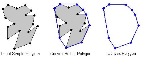
Figure X: The convex hull of a simple polygon. Notice how the rubber band encloses all points. — **Figure 1:** The convex hull of a simple polygon. Notice how the rubber band encloses all points (source).

On the left we have our original shape. And in the center we have the convex hull of original shape. Notice how the rubber band has been stretched to around all extreme points of the shape, but leaving no extra space along the contour — thus the convex hull is the minimum enclosing polygon of all points of the input shape, which can be seen on the right.

Another important aspect of the convex hull that we should discuss is the convexity. Convex curves are curves that appear to “bulged out”. If a curve is not bulged out, then we call it a convexity defect.

For example, take a look at the following hand-drawn image of a hand taken from the OpenCV documentation:

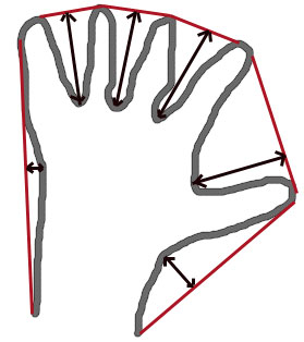
Figure X: Black arrows represent convexity defects of the hand image. — **Figure 2:** Black arrows represent convexity defects of the hand image.

The gray outline of the hand in the image above is our original shape. The red line is the convex hull of the hand. And the black arrows, such as in between the fingers, are where the convex hull is “bulged in” rather than “bulged out”. Whenever a region is “bulged in”, such as in the hand image above, we call them convexity defects.

Perhaps not surprisingly, the convex hull and convexity defects play a major role in hand gesture recognition, as it allows us to utilize the convexity defects of the hand to count the number of fingers. We’ll be exploring hand gesture recognition and convexity defects in Module 13 of this course.

But hand gesture recognition is not the only thing the convex hull is good for. We also use it when computing another important contour property: solidity.

Solidity

The last advanced contour I want to discuss is the solidity of a shape. The solidity of a shape is the area of the contour area divided by the area of the convex hull:

solidity = contour area / convex hull area

Again, it’s not possible to have a solidity value greater than 1. The number of pixels inside a shape cannot possibly outnumber the number of pixels in the convex hull, because by definition, the convex hull is the smallest possible set of pixels enclosing the shape.

Just as in the extent of a shape, when using the solidity to distinguish between various objects you’ll need to manually inspect the values of the solidity to determine the appropriate ranges. For example (and as we’ll see in the next sub-section), the solidity of a shape is actually perfect for distinguishing between the X’s and O’s on a tic-tac-toe board.

Getting Our Hands Dirty

So at this point we’ve reviewed some advanced contour properties such as aspect ratio, extent, convex hull, and solidity.

That’s great — but the real question is: How do we put these contour properties to work for us?

In the upcoming two sections we’ll be utilizing our contour properties to distinguish between X’s and O’s on a tic-tac-toe board and how to recognize different Tetris blocks. Both of these example problems are situations in which I’ve seen other computer vision programmers and developers immediately jump into using image descriptors and machine learning to solve these problems — that is simply overkill and is absolutely not necessary.

If anything, I want the key takeaway from this section to be: always consider contours before more advanced computer vision and machine learning methods.

Often (and as you’ll see below), a clever use of contour properties can enable us solve problems that may appear challenging on the surface, but are actually quite easy.

Distinguishing Between X’s and O’s

Let’s get started by recognizing the X’s and O’s on a tic-tac-toe board.

If you are unfamiliar with the game, the playing board looks like this:

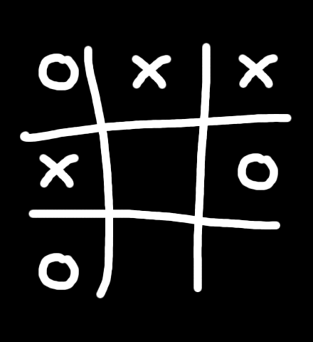
Figure 14: A tic-tac-toe game board. — **Figure 3:** A tic-tac-toe game board.

Tic-tac-toe is a two player game. One player is the “X” and the other player is the “O.” Players alternate turns placing their respective X’s and O’s on the board, with the goal of getting three of their symbols in a row, either horizontally, vertically, or diagonally. It’s very simple game to play, common among young children who are first learning about competitive games.

Interestingly, tic-tac-toe is a solvable game. When played optimally, you are guaranteed at best to win at and at worst to draw (i.e. tie).

While we aren’t going to dive into the game mechanics of optimal tic-tac-toe play, we are going to write a Python script that leverages computer vision and contour properties to recognize the X’s and O’s on the board. Using this script, you could then take the output and feed it into a tic-tac-toe solver to give you the optimal set of steps to play the game.

Anyway, enough talk. Let’s look at some code:

# import the necessary packages
import cv2
import imutils

# load the tic-tac-toe image and convert it to grayscale
image = cv2.imread("images/tictactoe.png")
gray = cv2.cvtColor(image, cv2.COLOR_BGR2GRAY)

# find all contours on the tic-tac-toe board
cnts = cv2.findContours(gray.copy(), cv2.RETR_EXTERNAL, cv2.CHAIN_APPROX_SIMPLE)
cnts = imutils.grab_contours(cnts)

# loop over the contours
for (i, c) in enumerate(cnts):
	# compute the area of the contour along with the bounding box
	# to compute the aspect ratio
	area = cv2.contourArea(c)
	(x, y, w, h) = cv2.boundingRect(c)

	# compute the convex hull of the contour, then use the area of the
	# original contour and the area of the convex hull to compute the
	# solidity
	hull = cv2.convexHull(c)
	hullArea = cv2.contourArea(hull)
	solidity = area / float(hullArea)

We’ll start off with our standard procedure of importing our necessary packages. Then we’ll load our tic-tac-toe game board (Figure 3) from disk and convert it to grayscale.

Line 10 handles finding the actual contours in the image. Notice how we are using the cv2.RETR_EXTERNAL flag in the cv2.findContours function to indicate that we want the external-most contours only.

Had we not provided this flag, we would have ended up detecting the inner circle of the “O” character as well as the outer circle! And if you don’t believe me, I would take a second a review the Finding and Drawing Contours section where we detail how to find contours in an image. Remember when we detected the contour of the inner-ovular region of the rectangle? The same premise applies here — if we were to detect all contours, we would end up finding the inner circle of the “O;” hence we are only interested in the external contours.

From there we start looping over each individual contour on Line 14.

And here is where we start computing the actual properties of our contour. We start off by computing the area of the contour on Line 17. Again, remember that the cv2.contourArea is not giving us the $area = width \times height$ area of the contour. Instead, it’s giving us the number of pixels that reside inside the contour (we’ll be computing the rectangular area of the contour later).

Line 18 then grabs the bounding box of the contour, which gives us the starting (x, y)-coordinates of the contour, followed by the width and height of the bounding box.

Given these two simple contour properties, let’s compute two advanced properties: the convex hull and the solidity. The actual convex hull of the shape is computed on Line 23 and the area of the convex hull is then computed on Line 24. Now that we have both the area of the contour along with the area of the convex hull we can compute the solidity, which we defined above.

So how are we going to put these properties to work for us? Let’s take a look:

	# initialize the character text
	char = "?"

	# if the solidity is high, then we are examining an `O`
	if solidity > 0.9:
		char = "O"

	# otherwise, if the solidity it still reasonabably high, we
	# are examining an `X`
	elif solidity > 0.5:
		char = "X"

	# if the character is not unknown, draw it
	if char != "?":
		cv2.drawContours(image, [c], -1, (0, 255, 0), 3)
		cv2.putText(image, char, (x, y - 10), cv2.FONT_HERSHEY_SIMPLEX, 1.25,
			(0, 255, 0), 4)

	# show the contour properties
	print("{} (Contour #{}) -- solidity={:.2f}".format(char, i + 1, solidity))

# show the output image
cv2.imshow("Output", image)
cv2.waitKey(0)

We’ll start by initializing our char variable to indicate the character that we are looking at — in this case, we initialize it to be a ? indicating that the character is unknown.

Lines 31 and 32 check to see if the character is an O — we hardcode a rule that if the solidity > 0.9 then, then character should be marked as an O.

And similarly, if the solidity > 0.5 (Lines 36 and 37) then we are examining an X.

Finally, if we are able to identify the character, we then draw the contour and the character on our image on Lines 40-43.

Intuitively, this makes sense. The letter X has four large and obvious convexity defects — one for each of the four V’s that form the X. On the other hand, the O has nearly no convexity defects, and the ones that it has are substantially less dramatic than the letter X. Therefore, the letter O is going to have a larger solidity than the letter X.

So how did I arrive that the solidity values of 0.9 and 0.5?

It wasn’t magic — I simply examined the solidity of each character on Line 46, which prints the solidity value and current contour ID to the screen.

Looking at the output of my terminal you can clearly see the ranges of valid values to distinguish between X’s and O’s:

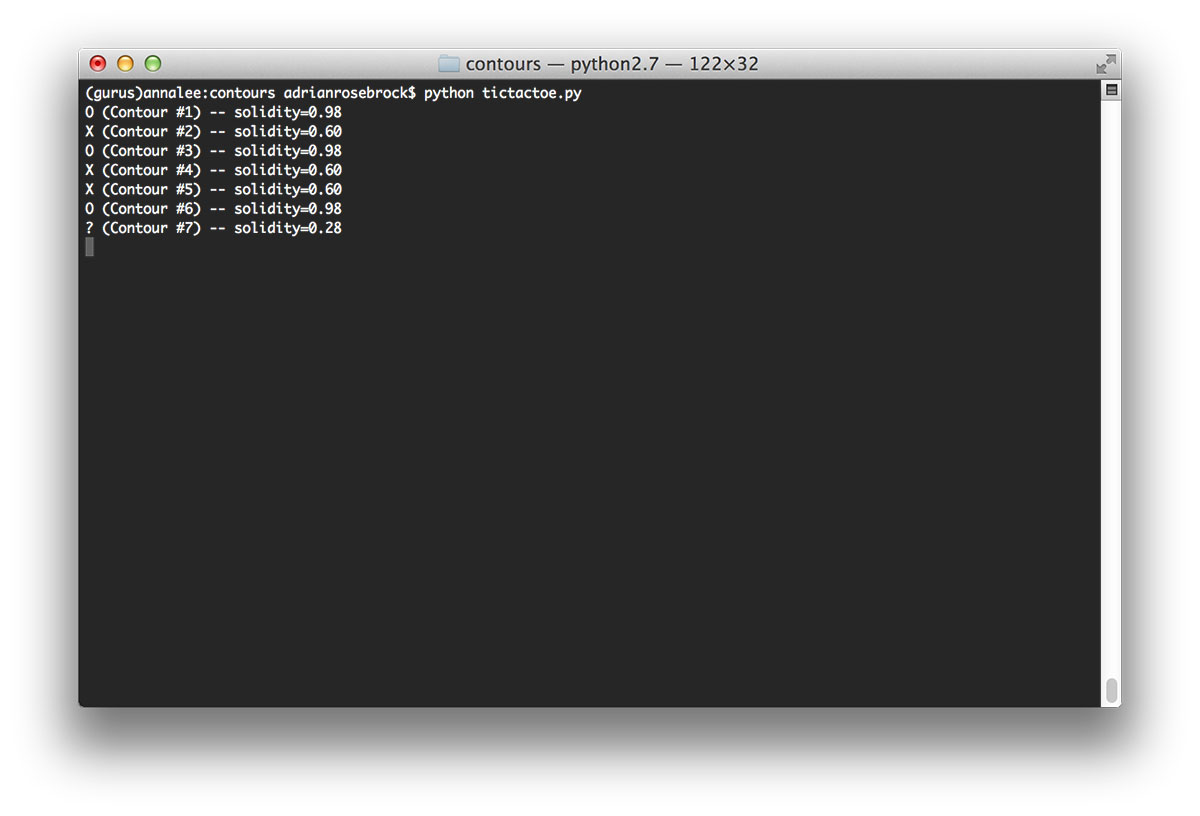
Figure 15: Examining the solidity value to define valid ranges for X's and O's. — **Figure 4:** Examining the solidity value to define valid ranges for X’s and O’s.

When we look at this output, we can see that the letter O has a solidity of 0.98 for all three times it appears on the board. Similarly, the letter X has a solidity of 0.6. The last solidity value of 0.28 refers to the actual game board itself.

Like I said, by inspecting these solidity values it becomes trivial to define the solidity value ranges to distinguish between X’s and O’s on Lines 31-37.

The actual output on a game board is thus:

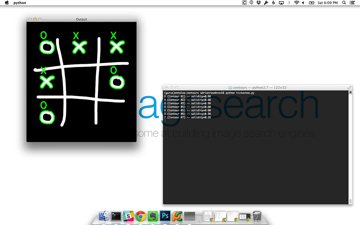
Figure 16: The final output of identifying X's and O's on a tic-tac-toe board. — **Figure 5:** The final output of identifying X’s and O’s on a tic-tac-toe board.

In this figure it’s substantially more clear that our algorithm is functioning as expected. We are able to identify all of the X’s and O’s without a problem while totally ignoring the actual game board itself. And we accomplished all of this by examining the solidity of each contour. No fancy computer vision algorithms. No fancy machine learning. Just leveraging contour properties to our advantage.

Identifying Tetris Blocks

Distinguishing between X’s and O’s in a tic-tac-toe game is a great introduction to the power of contour properties. But in the previous example we used only the solidity perform our identification. In some cases, such as in identifying the various types of Tetris blocks, we need to utilize more than one contour property. Specifically, we’ll be using aspect ratio, extent, convex hull, and solidity in conjunction with each other to perform our brick identification.

Open up a new file, name it contour_properties_2.py , and let’s start coding:

# import the necessary packages
import numpy as np
import cv2
import imutils

# load the Tetris block image, convert it to grayscale, and threshold
# the image
image = cv2.imread("images/tetris_blocks.png")
gray = cv2.cvtColor(image, cv2.COLOR_BGR2GRAY)
thresh = cv2.threshold(gray, 225, 255, cv2.THRESH_BINARY_INV)[1]

# show the original and thresholded images
cv2.imshow("Original", image)
cv2.imshow("Thresh", thresh)

# find external contours in the thresholded image and allocate memory
# for the convex hull image
cnts = cv2.findContours(thresh.copy(), cv2.RETR_EXTERNAL, cv2.CHAIN_APPROX_SIMPLE)
cnts = imutils.grab_contours(cnts)
hullImage = np.zeros(gray.shape[:2], dtype="uint8")

Again, we start with our standard practice of importing the necessary packages and loading our Tetris block image off disk.

Here is what our Tetris image looks like:

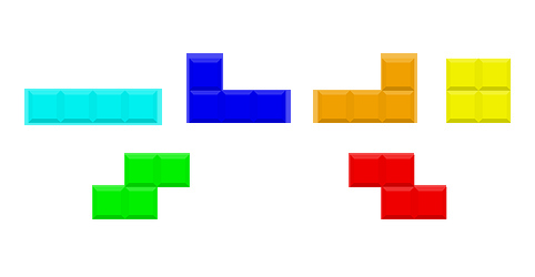
Figure 17: The Tetris blocks that we will be identifying. — **Figure 6:** The Tetris blocks that we will be identifying.

The aqua piece is known as a Rectangle. The blue and orange blocks are called L-pieces. The yellow shape is obviously a Square. And the green and red bricks on the bottom are called Z-pieces.

Our goal here is to extract contours from each of these shapes and then identify which shape each of the blocks are.

To accomplish this, we’ll need to create a binary image so we can extract the contours of the image. We apply thresholding on Line 10, which we covered in Module 1.8 to create a binary image, where the background pixels are black and the foreground pixels (i.e. the Tetris blocks) are white.

We then find the contours in our thresholded image on Line 18 and allocate a NumPy array with the same shape as our input image on Line 20 so we can visualize the convex hull of each shape. Visualizing the convex hull is not a required step in identifying the various Tetris blocks; however, I thought it would be interesting to include in this example so you could see what the contour of a convex hull looked like.

Let’s continue with our example:

# loop over the contours
for (i, c) in enumerate(cnts):
	# compute the area of the contour along with the bounding box
	# to compute the aspect ratio
	area = cv2.contourArea(c)
	(x, y, w, h) = cv2.boundingRect(c)

	# compute the aspect ratio of the contour, which is simply the width
	# divided by the height of the bounding box
	aspectRatio = w / float(h)

	# use the area of the contour and the bounding box area to compute
	# the extent
	extent = area / float(w * h)

	# compute the convex hull of the contour, then use the area of the
	# original contour and the area of the convex hull to compute the
	# solidity
	hull = cv2.convexHull(c)
	hullArea = cv2.contourArea(hull)
	solidity = area / float(hullArea)

	# visualize the original contours and the convex hull and initialize
	# the name of the shape
	cv2.drawContours(hullImage, [hull], -1, 255, -1)
	cv2.drawContours(image, [c], -1, (240, 0, 159), 3)
	shape = ""

On Line 23 we start looping over each of the contours individually so we can compute our contour properties.

We’ll start off by computing the area and the bounding box of the contour on Lines 26 and 27.

We then compute the aspect ratio, which is simply the ratio of the width to the height of the bounding box on Line 31. Again, remember that the aspect ratio of a shape will be < 1 if the height is greater than the width. The aspect ratio will be > 1 if the width is larger than the height. And the aspect ratio will be approximately 1 if the width and height are equal.

With this in mind, do you have any guesses as to what we’ll use the aspect ratio for?

If you guessed discriminating between the square and rectangle pieces, you would be correct. But more on that later.

Line 35 then computes the extent of the current contour, which is the area (i.e. number of pixels that reside within the contour) divided by the true rectangular (area = width x height) area of the bounding box.

Finally, Lines 40-42 compute the convex hull and the solidity in the same manner as we saw in the tic-tac-toe example.

We then visualize the convex hull, draw the current contour, and initialize the name of our shape on Lines 46-48.

Now that we have computed all of our contour properties, let’s define the actual rules and if statements that will allow us to discriminate between the various Tetris blocks:

	# if the aspect ratio is approximately one, then the shape is a square
	if aspectRatio >= 0.98 and aspectRatio <= 1.02:
		shape = "SQUARE"

	# if the width is 3x longer than the height, then we have a rectangle
	elif aspectRatio >= 3.0:
		shape = "RECTANGLE"

	# if the extent is sufficiently small, then we have a L-piece
	elif extent < 0.65:
		shape = "L-PIECE"

	# if the solidity is sufficiently large enough, then we have a Z-piece
	elif solidity > 0.80:
		shape = "Z-PIECE"

	# draw the shape name on the image
	cv2.putText(image, shape, (x, y - 10), cv2.FONT_HERSHEY_SIMPLEX, 0.5,
		(240, 0, 159), 2)

	# show the contour properties
	print("Contour #{} -- aspect_ratio={:.2f}, extent={:.2f}, solidity={:.2f}"
		.format(i + 1, aspectRatio, extent, solidity))

	# show the output images
	cv2.imshow("Convex Hull", hullImage)
	cv2.imshow("Image", image)
	cv2.waitKey(0)

As I hinted at above, if the aspect ratio of a shape is approximately 1, then the width and height of the shape are roughly equal. And if this is the case, we know that in context of our Tetris blocks, if the width and height are equal, then we must be examining a square (Lines 51 and 52).

Similarly, if the aspect ratio is large, then the width is much greater than the height. And in the context of identifying Tetris pieces, this must mean we are examining a horizontal rectangle (Lines 55 and 56).

However, if the rectangle was vertical rather than horizontal, the aspect ratio would then be very small since the height would be substantially larger than the width. I did not account for this in the code above and I’ll leave it as an exercise for you to convince yourself of this point (it’s good to have a little homework).

Finally, Lines 59 and 60 examine the extent to see if we are looking at an L-piece, and Lines 63 and 64 check to see if we are examining at Z-piece. Again, just like in the tic-tac-toe board, I manually investigated the values of the aspect ratio, extent, and solidity to define the valid ranges to distinguish between the Tetris block pieces — and if you were developing your own shape identification script, you would have to perform the same type of investigation. This will become very obvious once we look at the output of our Python script.

We then draw the name of the shape on our image on Lines 67 and 68, print our contour properties to our terminal on Lines 71 and 72, and display our output images to screen on Lines 75-77.

To execute this script, simply navigate to our source code directory and execute the following command:

$ python contour_properties_2.py

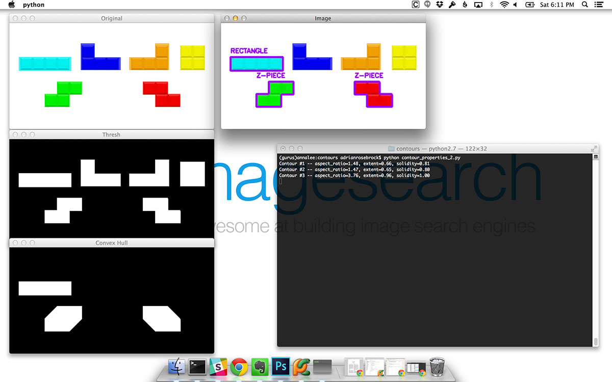
Once the script executes, you’ll see the first image popup on your screen:

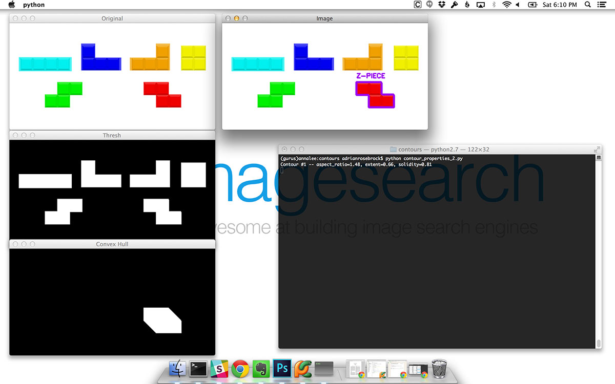
Figure 18: Identifying the first Z-piece using contour properties. — **Figure 7:** Identifying the first Z-piece using contour properties.

On the top we have our original input image. Below that we have our thresholded image (Line 10) where the actual Tetris blocks we want to identify appear as white on a black background. And then on the bottom we have our convex hull image for the Z-piece — notice how this shape almost looks like a skewed hexagon. This is because the convex hull is accounting for the two convexity defects (i.e. where the Z-piece is “bulged in”).

Then, looking at the output of the terminal we see that the solidity is >= 0.8 — according to our rule, this must be a Z-piece.

Let’s look at the next shape:

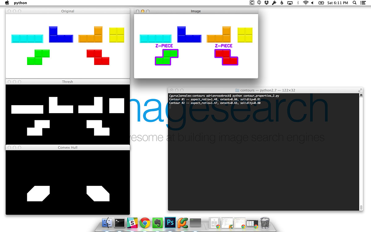
Figure 19: Identifying the second Z-piece. — **Figure 8:** Identifying the second Z-piece.

Again, we are applying the same thought process as in the previous figure. We can see that the solidity of the shape is also >= 0.8, thus we are once again examining a Z-piece.

Figure 20: Identifying the rectangle Tetris block. — **Figure 9:** Identifying the rectangle Tetris block.

Identifying the rectangle Tetris block is very easy — since the block is so elongated, the width is substantially larger than the height. This means that the aspect ratio must be quite larger. In this case the aspect ratio = 3.76, allowing our rule on Line 55 to correctly identify the shape as a rectangle.

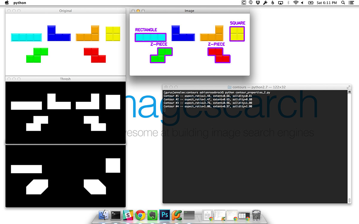
Figure 21: Identifying a shape using the aspect ratio is trivially easy. — **Figure 10:** Identifying a shape using the aspect ratio is trivially easy.

Just like identifying the rectangle in Figure 9 above was easy, recognizing the square is even easier. Since a square has (approximately) the same width and height, we know that if the aspect ratio = 1, (plus or minus some $\epsilon$ , of course) the shape must be a square.

Also take a look at the visualization of the convex hull for both the rectangle and the square. Since both the rectangle and square shapes have no convexity defects, the convex hull is actually no different than the original shape.

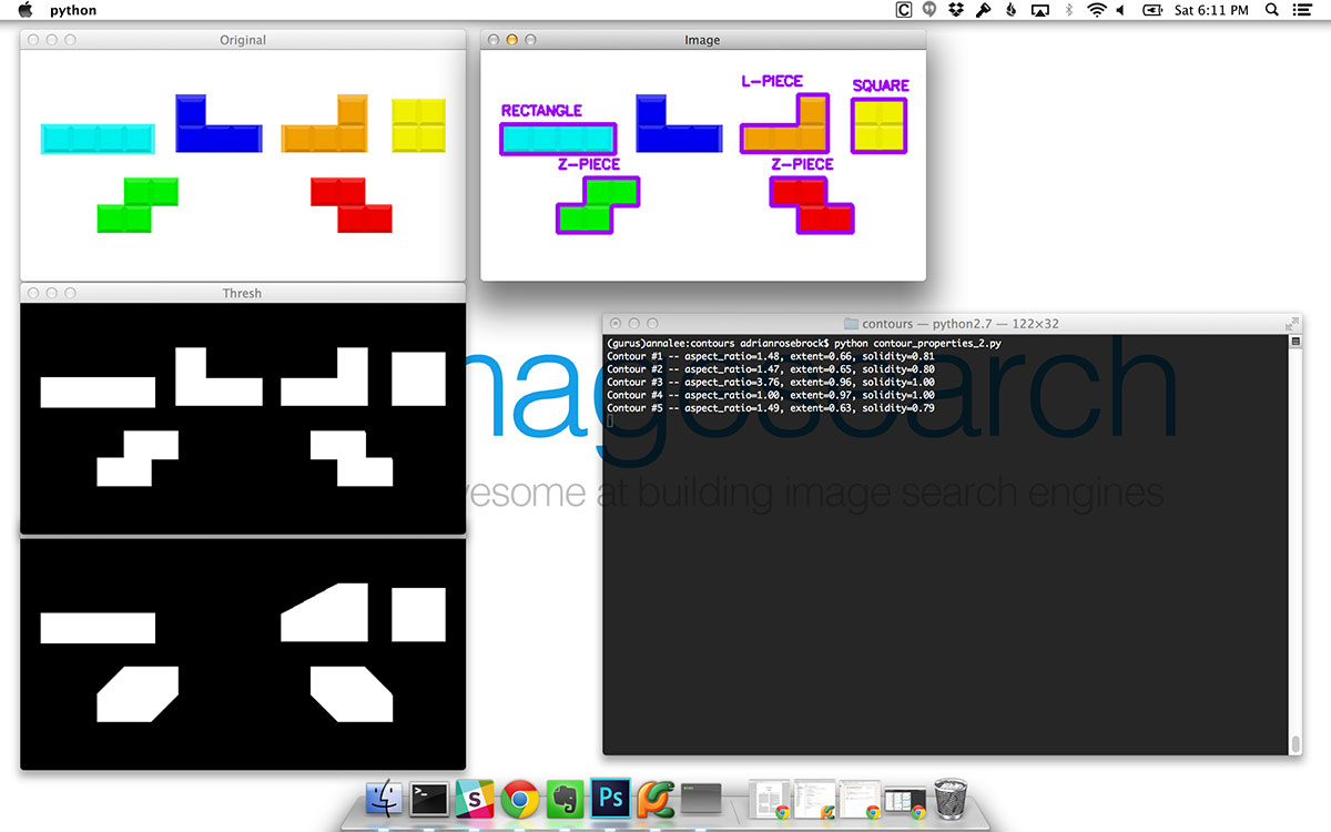
Figure 22: Identifying the first L-piece using the extent. — **Figure 12:** Identifying the first L-piece using the extent.

Take a look at the output of our terminal. Up until Contour #5, has the extent of a shape dipped below 0.65? According to our output, it has not. Thus, the extent is a good property to distinguish the L-piece.

The same is true for the second L-piece below:

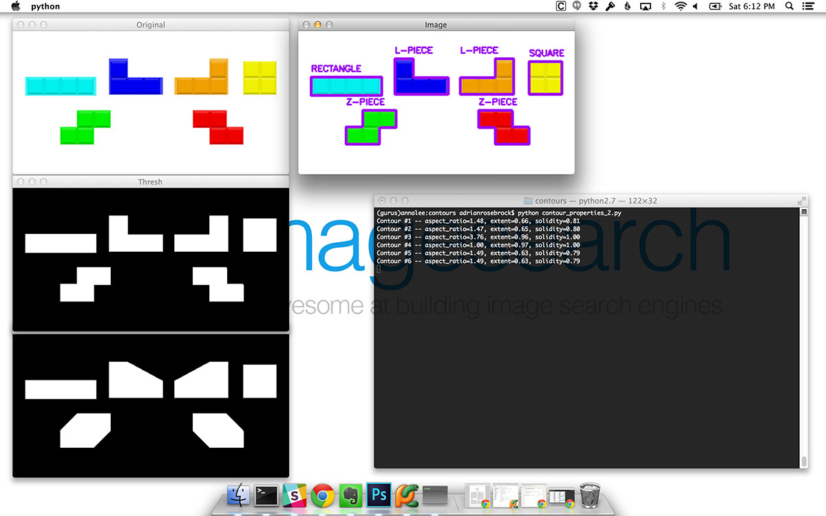
Figure 23: Identifying the second L-piece using the extent. — **Figure 13:** Identifying the second L-piece using the extent.

As you can see, using nothing more than the aspect ratio, extent, and solidity of a shape we were able to distinguish between the four different types of Tetris blocks.

Of course, there is more than one way to skin this cat. We could have also used methods to quantify and represent the shapes, like Hu moments or Zernike moments, which we’ll cover later in this course.

But at the same time, why bother?

Using simple contour properties, we were able to recognize X’s and O’s on a tic-tac-toe board. And we were also able to recognize the various types of Tetris blocks. Again, these contour properties, which are very simple on the surface, can enable us to identify various shapes — we just need to take a step back, be a little clever, and inspect the values of each of our contour properties to construct rules to identify each shape.

Summary

In this lesson we built upon our previous simple contour properties and learned about more advanced contour properties such as aspect ratio, extent, convex hull, and solidity.

Using these contour properties then enabled us to distinguish between X’s and O’s on a tic-tac-toe board and recognize various Tetris block pieces. Again, these shape identifications were accomplished using only contour properties. We did not have to apply any type of advanced techniques such as machine learning or training our own object classifier to obtain our shape classifications.

Downloads:

Download the Code